Optimization - Breault Research Organization, Inc.

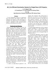
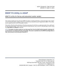
ASAP TECHNICAL PUBLICATIONBRO4309 (AUGUST 26, 2009)OptimizationGeneral-purpose optimization methods in ASAPThis technical publication describes enhanced optimization capabilities and the process for effectively using themin the Advanced Systems Analysis Program (ASAP®) from Breault Research Organization (BRO). New capabilitiesfor optimization were introduced in ASAP 2009, and are in addition to pre-existing optimization capabilitiesin ASAP. This publication complements optimization topics in ASAP HTML Help for this release.BACKGROUNDThe process of optimization, or minimization, in optical system design takes a set of the system’s defining parameters,such as surface curvatures, conics, optical properties, and so on, and systematically varies their values toreach a desired result, usually measured in terms of the distribution of energy at specified locations within the system.The system parameters that are adjusted are called variables, and the description of the desired system performanceis referred to as the merit function.The optimal solution, called the global minimum, consists of the set of variable values that locate the system thathas the smallest value for the merit function that can be attained. Most systems have a range of potential solutionscalled local minima. Any system can have only one global minimum. In many situations, it is not possible to determinethat a given solution is the global minimum. However, in most instances it is only necessary to locate asolution that meets the system requirements within some specified range.ASAP provides the structure for enhanced optimization capabilities. Included in ASAP are three general-purposeoptimization methods:• Brent’s Method• Downhill Simplex• Simulated AnnealingEach method is effective in finding optimal solutions for many different imaging and illumination systems. A briefdescription of each method is included in this section. Other sections, including “Selecting the optimization method”on page 11 and “Examples of optimization methods” on page 19 discuss using the optimization user interface.Breault Research Organization, Inc.Copyright © 2006-2014 All rights reserved.6400 East Grant Road, Suite 350, Tucson, Arizona 85715 USAwww.breault.com | info@breault.com800-882-5085 USA | Canada | 1-520-721-0500 Worldwide | 1-520-721-9630 Fax

OptimizationBrent’s methodBrent’s method is a technique for finding the minimum value of a function in a one-dimensional solution space(that is, only one variable). This technique combines several root-finding algorithms to form a very fast and robustoptimization technique as long as the solution space is not discontinuous.Downhill simplex methodThe Nelder-Mead method uses a simplex to find the minima of an N-dimensional function, where N is the numberof variables. The simplex is defined by N+1 vertex points. In two dimensions, the simplex has the form of atriangle formed on a plane. In three dimensions, the simplex is tetrahedral.The downhill simplex method solves for the minimum solution of a continuous solution space by evaluating thefunction at the vertex locations and then adjusting the orientation, size or shape of the simplex based on thesevalues. After each modification of the simplex, the merit function is reevaluated at the new vertex locations, resultingin a further change to the simplex. This method is useful for finding a local minimum solution for situationswhere the merit function is smooth and continuous. Modifying the simplex near the local minimum has thepotential to move the solution away from a local minimum in an attempt to find the location of a better minimum.Simulated annealing methodSimulated annealing is an optimization technique that attempts to mimic the physical process of annealing materialssuch as metals or glass. Annealing is used to form materials with improved physical properties.Three steps in the annealing process are:1 Heating the material to the annealing temperature,2 Holding the material at this temperature until it is uniformly heated, and3 Cooling the material at a predefined rate to allow for the optimal orientation of atoms andmolecules.The optimal orientation is the distribution that requires the least energy to maintain. In applying this process tooptimization, the various systems (variables and their associated values as well as the resulting merit functionvalue) are analogous to the equivalent states of the annealing material. The merit function defines the “energystate” of a particular solution.A control parameter—the temperature—is used to limit the acceptable range of solutions. If the temperature isrelatively large, solutions that result in a higher energy state may be accepted, as they may indicate a path to amore optimal state. As the temperature is reduced, the allowed range of positive departure in the merit functionis reduced and as the temperature approaches zero, only solutions resulting in a lower merit function are accepted.As a local minimum is achieved, the system is perturbed to a random starting point and the process runs again,looking for a different, possibly better local minimum.2 Optimization

. . . . .OPTIMIZATION PROCESSThese are the steps involved in setting up ASAP to perform optimization. Each step is described in detail in this section.1 Define the system in ASAP2 Define design variables3 Define design objectives4 Define objective constraints5 Select the exit criteria6 Select the optimization methodDefining the system in ASAP• Optimization can be performed on almost any ASAP INR file. Before using the file for optimization, makesure that the file runs to completion without error. If you modify a file after you open it, the file must besaved before optimization. Changed files are indicated in ASAP Workspace by an asterisk (*) after the filename.• The optimization takes less time if any unnecessary graphical calculations are removed or “commented out”of the script before beginning the optimization process.• Limit the extent of the solution search by starting with a “reasonable” design. This includes making sure thedesign can be ray traced to the surfaces of interest with reasonable efficiency. For example, if a design goalis to maximize energy on a detector and in the baseline design, little or no energy reaches the detector, ASAPcan not readily determine the effects of parameter changes on the detector energy without requiring the userto define very complex, time-consuming merit function to distinguish the actual rays reaching the surface ofinterest. Optimization in ASAP is a tool to help optical or illumination designers do their job. It is notintended to do the job of the designer.• The file must include command lines identifying available design variables, objectives, and constraintsusing the form name=value.After the script file is modified and saved, the optimization process can be started by selecting Optimize Scripton the Optimize menu on the main menu bar. This opens the Optimization Setup Summary window, shown inOptimization 3

OptimizationFigure 1. Each tab on this window is addressed separately in this section.Figure 1 Optimization Setup Summary window (without entries)DEFINING DESIGN VARIABLES• Any system parameter can be used as a design variable by including a variable definition command in theINR file.• Each variable must be defined on a separate line. Comments are allowed on variable lines or between linesof variables, but variable definitions cannot be combined on a single line with a semicolon (;).• To add a variable to the variable list, select the text in the INR file, right-click the highlighted text, and selectDefine Design Variable on the shortcut menu or use the Optimize menu. Follow the same procedure toselect any variables that may be used during the optimization. Variables must be defined using the formname=value. Multiple variables that are listed on sequential lines in the INR file can be selected together bypressing the Shift key while selecting the first and last listed variables.4 Optimization

. . . . .• The name and nominal value of each selected variable is displayed on the Design Variables tab of theOptimization Setup Summary window, shown in Figure 2. To make a variable easier to identify, you canoptionally assign a pseudonym to the variable in the Alias column.Figure 2 Sample entry on the Design Variable tab• Columns limit the range of allowed values for each variable. Brent’s method requires initial bounding ofparameters. If you do not provide these as input, ASAP “guesses” at proper limits, which may possiblyresult in a non-optimal solution. With all optimization methods, setting reasonable bounds, based on anunderstanding of the system’s requirements, results in more effective optimization.• The step size, if entered, must be a value less than the difference between the maximum and minimumvalues. This value is used by ASAP to help determine initial movements in variable space.• The manufacturing tolerance is used to restrict solutions to the manufacturing limit.Optimization 5

Optimization• The Enabled State column includes a drop-down list for including (enabling) and removing (disabling)individual variables from the optimization. You can add all potential variables to the dialog, disabling someof them until later in the optimization process. Enabling and disabling variables can be used to determinewhich variables are most effective for a particular design.• The Current column lists the value currently associated with each variable.• For further information on this tab, select Help to open the topic, “Optimization Design Variables Tab” inASAP Help.DEFINING DESIGN OBJECTIVESDesign objectives describe the goals of the design. The total of the design objects is called the merit function.• To add a design objective, select the text in the script file for the objective, right-click the highlighted text,and select Define Design Objective on the shortcut menu or use the Optimize menu. Follow the sameprocedure to select other objectives that may be used during the optimization. Objectives must be definedusing the form name=expression. Multiple design objectives that are listed on sequential lines in the INRfile can be selected together by pressing the Shift key while selecting the first and last listed objectives. Eachdesign objective must be defined on a separate line. Comments are allowed on variable lines, but variabledefinitions cannot be combined on a single line with a semicolon (;).• The goal of the optimization is to minimize the system figure of merit, which is the squared-sum of thedifferences between the value of each design objective and its target value, multiplied by a weighting factor.Target values and weighting factors can be entered in the appropriate columns of the Design Objectives tabof the Optimization Setup Summary window, shown in Figure 3. Default target values are 0 and the defaultweighting factors are 1. Design objectives can be directly constructed in the merit function to include theeffects of non-zero targets and non-uniform weighting, if desired.• The Enabled State column includes a drop-down list for including (enabling) and removing (disabling)individual design objectives from the optimization. The current values associated with each objective arereported during the optimization, even if it is disabled, but it is not included in the calculation of the system’sfigure of merit.6 Optimization

. . . . .• For further information on this tab, select Help to open the topic, “Optimization Design Objectives Tab” inASAP Help.Figure 3 Sample entries on the Design Objectives tabDEFINING OBJECTIVE CONSTRAINTS (OPTIONAL)Objective constraints are used to force system parameter or analysis result to be within a bounded range. Objectiveconstraints are not required.• To add an objective constraint, select the text in the script file for the objective constraint, right-click thehighlighted text, and select Define Objective Constraint from the menu. Follow the same procedure toselect other objective constraints that may be used during the optimization. Objective constraint must bedefined using the form name=value.• The Minimum and Maximum columns on the Objective Constraints tab of the Optimization Setup Summarywindow are used to set the limits for the constrained item. These values are optional. This allows for singlesidedconstraints, such as item value is not greater than the set maximum value, with no minimum limit. SeeFigure 4.• The Enabled State column includes a drop-down list for including (enabling) and removing (disabling)individual objective constraints from the optimization.Optimization 7

Optimization• For further information on this tab, select Help to open the topic, “Optimization Constraints Tab” in ASAPHelp.Figure 4 Sample entries on Objective Constraints tabDEFINING AND ASSIGNING A PENALTY FUNCTION (OPTIONAL)When a penalty function is assigned to an enabled objective constraint, ASAP applies the penalty function to theFigure of Merit during any iteration of the script in which the constraint is violated. You can define penalty functionsbefore or after defining objective constraints, but a penalty function can be assigned only after an objectiveconstraint is define. Penalty functions are entered as separate items in the ASAP script in the formname=expression.• To define a penalty function for a constraint, select a penalty function from the script, and select DefinePenalty Function from the context menu by right-clicking the Editor window, or from the Optimize menu.The selected text should contain the name of the penalty function and its value.8 Optimization

. . . . .• To assign a penalty function to a defined objective constraint, select the name of the constraint on theObjective Constraints tab, and select a pre-defined penalty function name from the drop-down menu in thePenalty Functions column on the same row.• To remove a penalty function from a constraint, select No Penalty Functions Assigned from the dropdownmenu in the Penalty Function column on the same row as the constraint. Defined constraints can beenabled or disabled, and penalty functions can be assigned or unassigned.TIP For a more detailed description, see the Knowledge Base for the technical publication, “Optimization- Penalty Functions, Solving constrained optimization problems”,http://www.breault.com/k-base.php?kbaseID=252.SELECTING EXIT CRITERIADuring optimization, ASAP attempts to find the solution resulting in the smallest figure of merit. The result is afunction of the starting parameter values as well as any limits placed on the design. In almost all instances, it isnot possible to know whether the optimal solution found is a local minimum or the global minimum.After determining the location of a minimum solution, ASAP perturbs the system to start another search of solutionspace, and continues this process until stopped. For this reason, it is always necessary to define an exit criterionon the Exit Criteria tab of the Optimization Setup Summary window, which triggers ASAP to stop theOptimization 9

Optimizationoptimization. See Figure 5.Figure 5 Sample entries on the Exit Criteria tab• The default exit criterion is a limit on the number of trials of 100. You can modify the number of trials to beany integer value greater than 0. A limit on the number of trials is always required.• The Use Acceptance Limit option defines the maximum level for an acceptable solution. Optimizationstops when a solution with a figure of merit less than the acceptance level is found.• During optimization, ASAP may select trial solutions that result in degraded performance (higher figure ofmerit), since these solutions may lead to solution paths with improved performance. The RelativeDivergence of Trials option triggers a termination of optimization if the solutions are diverging faster than auser-specified rate over a user-specified number of trials.10 Optimization

Optimization• The Downhill Simplex method is appropriate for systems where the merit function is smooth andcontinuous. Select the Advanced Options button on the Optimization Method tab of the Optimization SetupSummary window to modify the scaling parameters used to resize and reposition the simplex. See Figure 7.Figure 7 Sample parameter entries for Downhill Simplex method12 Optimization

. . . . .• The Simulated Annealing method is appropriate for situations when the merit function may havediscontinuities or it is necessary to sample wide ranges of solution space.• The Initial Temperature is used to establish the scale of solution space. The selection of Geometric orPower Law determines the rate of cooling of the system. At higher temperatures, a wider range of solutionsare explored in an attempt to find the optimal design. As the system cools, only solutions resulting inimproved figure of merit values are accepted. The block size parameter defines the rate (number of trials) atwhich the temperature is adjusted. No one temperature is best for all systems. A temperature of 0 results indownhill simplex optimization. See Figure 8.Figure 8 Sample parameter entries for Simulated Annealing method• For further information on this tab, select Help to open the topic, “Optimization Method Tab” in ASAPHelp.Optimization state fileThe Optimization feature in ASAP includes a provision for saving the current state of the optimization in a textfile referred to as an optimization state file (OSF). The OSF file can be saved anytime after the optimization hascompleted at least one optimization cycle. It contains information identifying design variables with values, constraints,and any other user-specified limit; design objectives with target, weight and enabled state; objectiveconstraints and associated penalty functions; selected exit criteria; as well as the applied optimization methodwith associated parameter values.Optimization 13

OptimizationThe OSF file also contains information about the figure of merit for all trial systems that were identified prior tohalting the optimization.You can use a saved OSF file to re-initiate the optimization process without needing to redefine any of the optimizationinputs. The OSF logs the current state of the merit function and optimization status, and can be automaticallyupdated, saved, and read into current and subsequent optimization processes.GENERATING AND SAVING AN OPTIMIZATION STATE FILETo generate an OSF:1 Start with an ASAP file suitable for optimization.2 Define all desired parameters on the Optimization Setup Summary window. These can includeboth enabled as well as disabled parameters.3 Set an exit criteria and start the optimization, using the desired optimization method.14 Optimization

. . . . .You can generate the OSF after the optimization is halted by either reaching a natural stopping point in the optimization(for example, after exhausting the desired trials), or when you halt it after some number of trials.Figure 9 Saving a set of optimization trials to an Optimization State FileThe option to generate the OSF file is found on the Optimize menu. To access the Optimize menu, you may needto select the name of the optimized file in the ASAP Workspace window.4 On the Optimize menu, select Save Optimization State.5 Select Save and accept the default name or enter the file name. By default, the file is saved inthe current ASAP working directory.NOTE No editing can be done on the ASAP file. However, you can edit the Optimization Setup Summarywindow.The OSF file contains optimization information in a structured format. This text file can be opened in any externaltext file editor. The initial part of the file contains the original ASAP script, followed by a listing of the statusOptimization 15

Optimizationand properties of all the optimization parameters. A partial file is shown in Figure 10.Figure 10 Sample optimization state file (*.osf)USING AN OPTIMIZATION STATE FILETo resume an optimization from a previously saved state, simply load an OSF file into ASAP. Select File, Open,and select the OSF file. The file opens in optimization mode, and the Optimization Setup Summary window is16 Optimization

. . . . .displayed. In this state, optimization elements on the tabs (design variables, objectives, and so on) can be addedor deleted, enabled or disabled.Figure 11 Open OSF file showing initial variable valuesEach of the tabs on the displayed Optimization Setup Summary window contains the parameters defined duringthe initial optimization setup. The nominal value for each of the design variables is changed to indicate the variablevalues for the final system evaluation of the saved optimization run. Before resuming the optimization,make any desired changes within this window, and then select Start Optimization on the Optimization Methodtab. The Optimization Results window is quickly populated with stored results from prior optimizations, andthen resumes the optimization according to the current state of the Optimization Setup Summary window.OPTIMIZATION SCRIPT LIBRARIESASAP users often create libraries of commonly used command sequences for frequently performed analyses.Whenever the desired function is required, the ASAP script can be reused. Similarly, a user may develop a libraryof useful optimization scripts; in particular, sets of design objectives that may be commonly used. An exampleof this might be an extensive set of test point values for an automotive headlamp.The OSF file is designed to allow you to generate a new OSF file outside of ASAP. It appends the informationthat defines the design objective or variables directly into an existing ASAP script file.Optimization 17

OptimizationNOTE If you generate an OSF externally of the ASAP optimization feature, you must follow the requiredformat. A missing parameter (such as an uninitialized variable) is ignored by ASAP, which could result ininaccurate optimization results.See “Examples of optimization methods” on page 19.18 Optimization

. . . . .EXAMPLES OF OPTIMIZATION METHODSBrent’s method exampleBrent’s method is used for systems where there is only one variable. This form of optimization may be usefulfor tolerance analysis of single compensator systems and for simple optimization of surface shape. We look atthe optimization to determine the appropriate parabola to form an image at a given location.A parabolic surface is a conicoid of revolution. It is rotationally, but not spherically symmetric. The parabola canbe defined in several forms. Typically, it is defined by a radius of curvature (or curvature) as well as a conic constantthat exactly equals -1. It can also be defined as a polynomial function, as shown in Equation 1.Equation 1where z is the surface sag and x and y are the surface coordinates. This can be described using the GENERALsurface:X2 (A)Y2 (A)Z 1SURFACEGENERAL 0 0 0Optimization 19

OptimizationParabolas are used to focus incident collimated light or to collimate light incident from a small source located atthe focus. See Figure 12.Figure 12 Parabola used to focus collimated lightWe demonstrate Brent’s method by finding the coefficient value for a parabola of a required focal length. Thestarting design is shown in Figure 13.Figure 13 Parabola design starting point20 Optimization

. . . . .Notice that the parabola is aiming the light towards the detector surface on the left.1 If you modified the ASAP script file, save it, and then select Optimize Script on the Optimizemenu.The Optimization Setup Summary window opens.2 Select the row in the ASAP script indicating the variable, right-click the highlighted text, andselect Define Design Variable.Notice that the surface definition references the variable identifier, shown in Figure 14.Figure 14 ASAP script defining variable and surface3 Set an appropriate minimum and maximum value.For example in this case, a positive coefficient causes the light to converge towards the detector surface, so weknow that the coefficient should not be negative. Design experience and intuition play an important role in settingup a proper optimization. See Figure 15.Figure 15 Initial design variable and limitsOptimization 21

OptimizationThe design objective is to minimize the RMS spot size on the detector. The necessary ASAP script is shown inFigure 16.Figure 16 Design objective definition in ASAP script4 Select the row in the script that defines the term size, right-click and select Define DesignObjective, and accept the default target and weight values. See Figure 17.Figure 17 Set design objectivesNo objective constraints are necessary for this problem.5 Accept the default of 100 trials on the Exit Criteria page.Brent’s method is the only allowable optimization technique.6 Change the Optimization Session Title if desired, and then select Start Optimization.22 Optimization

. . . . .The optimization rapidly converges to the solution. In this case, the local optimum is also the global optimum.See Figure 18.Figure 18 Optimization trial dataOptimization 23

Optimization7 Select any trial solution row and the select Save System Under Evaluation on the Optimizemenu. See Figure 19.This step saves a copy of the optimized file using the variable value of the specified trial. The information aboutall of the trials is saved to the working directory.Figure 19 Create a file, based on a selected trial solution, via the Save System Under Evaluation command onthe Optimize menu24 Optimization

. . . . .8 Select the Close button on the Optimization Setup Summary window, and run the saved file,which is listed under the INR Input section of the ASAP Workspace. See Figure 20.Figure 20 Optimized design outputOptimization 25

OptimizationDownhill simplex exampleFor the downhill simplex example, assume an illumination system is desired, which maximizes the light capturedon a screen at some distance. In addition to capturing most of the energy, it is desired that the illumination patternappears uniform and square. Use of the optics to help shape the illumination pattern increases the system efficiency,since an aperture is not used to block valuable energy.Begin by applying design knowledge to determine a reasonable starting point. We need a distribution that hasquadrant symmetry, that takes light from a source, and spreads it out to a desired size and shape. A parabola withthe source gives a diverging distribution that is rotationally symmetric. We can get the desired symmetry by expandingthe GENERAL surface definition to include additional terms. Start with one additional coefficient beyondthe parabola on the x^2*y^2 term.X2Y2SURFACE(A)(A)GENERAL 0 0 0X2Y2 (B)Z 1In terms of the design objectives, an extended source launching a large number of rays can be used. The meritfunction can then target the energy in a range of pixels, as well as the differences between the energy in eachpixel. Although this works, there is significant ray tracing overhead. If we consider the problem at the simplestlevel, we are trying to map a circle at the optic onto a square at the detector. We need to define a merit functionthat performs this mapping. We need to use a sufficient number of rays to define our target. Because of the system’ssymmetry, we need to target rays only in one quadrant. Three rays are mapped from the edge of the circleto the edge of the square, and three are mapped from the middle of the circle to the middle of the square. See26 Optimization

. . . . .Figure 21.Figure 21 Mapping of source to imageThese rays can be used to perform the necessary mapping. See Figure 22.Figure 22 Source rays used to perform mapping1 Select initial parameter values so that all rays land on the detector surface.Optimization 27

OptimizationThis provides a reasonable starting point for the design. See Figure 23.Figure 23 Starting design - one example2 Define the design variables. See Figure 24.Figure 24 Table of design variables28 Optimization

. . . . .3 Define the design objectives. See Figure 25.The FLX objective is included, but disabled, so that it can be tracked during the optimization, but it is not includedin the figure of merit calculation. When using downhill simplex, try to avoid objectives that may introducediscontinuity into the merit function.Figure 25 Table of design objectivesNo design constraints are necessary for this example.4 Set the exit criteria to 50 trial solutions.5 Select the Downhill Simplex Method using the default control parameters, and select the StartOptimization button.Optimization 29

OptimizationThe optimization quickly finds an optimal region of solution space, isolates the local minimum, and proceedsthrough the requested number of trials. If more trials were designated, the optimizer would restart the search ina different parameter space. See Figure 26.Figure 26 Optimization results30 Optimization

. . . . .One of the trial solutions is saved and run to view the results. The location of the six targeted rays is shown inFigure 27.Figure 27 Ray locations on detectorOptimization 31

Now look at the design with a more realistic extended source. See the original system in Figure 28, and see theoptimized system in Figure 29.Figure 28 Starting design—original system

. . . . .Figure 29 Optimized systemIn addition to saving an individual optimized system (Save System Under Evaluation), ASAP automaticallysaves information and all session trials in a text file that was identified by the user-entered Optimization SessionTitle on the Optimization Method tab of the Optimization Setup Summary window. Variable value informationfrom any of the trials is found in this file, and can be entered into ASAP for further analysis, or the entire file canbe opened in a program such as a spreadsheet for post-processing.Optimization 33

OptimizationThe Print Report option is also available on the Optimize menu. If you select this option, the Print Report dialoggives you the choice of printing the entire optimization summary or only one selected system. See Figure 30.Figure 30 Print Report dialog to select the print range34 Optimization

. . . . .You can also choose to print the graph of the Figure of Merit vs. Trial Solution. Printed output is shown in Figure31 and Figure 32.Figure 31 Print report of entire systemFigure 32 Print report of selected systemOptimization 35

Optimization9 Accept the default parameter values for the power law.10 Select the Start Optimization button. See Figure 36.Figure 36 Sample entries for Simulated Annealing method38 Optimization

. . . . .The optimization quickly found the region of optimal performance, but the shape of solution space provides alarge number of local minima in the region. See the optimization results in Figure 37.Figure 37 Results of optimization in solution space and tabular layout11 Save one of the optimized trials for further analysis.For this design, the coupling efficiency is 88%. See Figure 38.The simulated annealing process automatically restarts after determining a local minimum has been located inan attempt to find a better solution. When this occurs, a message is sent to the Command Output window. SeeFigure 38.Optimization 39

OptimizationFigure 38 Coupling efficiency and parameters of optimized designCONCLUSIONThe general nature of the optimization methods in ASAP makes this tool useful for optimizing a wide range ofoptical and illumination systems.40 Optimization