BSL PRO Lesson H32 - Biopac

Updated 7.20.12
BSL PRO Lesson H32:
Heart Rate Variability Analysis
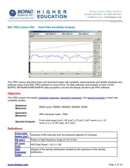
This PRO Lesson describes basic and advanced heart rate variability measurements and details hardware and
software setup of the BSL PRO software to record ECG. All data collection and analysis is done via the
BIOPAC MP36/MP35/MP30/MP45 data acquisition unit and the Biopac Student Lab PRO software.
Objective
This PRO Lesson will explain statistical measures, geometric measures, and spectral analysis in heart rate
variability studies.
Statistical
Measures:
Geometric
Measures:
Spectral Analysis:
NN50 count, PNN50, RMSDD, SDANN, SDSD
HRV triangular index, TINN
5-min total power (ms ), HF (ms 2 ), LF (ms 2 ), HLF morm (n.u.), LF
norm (n.u.), LF.HF ratio, VLF (ms 2 )
Definitions
5-min total
power (ms )
HF (ms 2 )
HF norm
(n.u)
HRV
triangular
index
Variance of NN intervals over the temporal segment (5 minutes).
Power in high frequency range (0.15-0.4 Hz)
HF/(Total Power - VLF) x 100
Integral of the density distribution divided by the maximum of the density
distribution.
www.biopac.com Page 1 of 16

BSL PRO Lesson H32
BIOPAC Systems, Inc.
LF norm
(n.u.)
LF/(Total Power - VLF) X 100
LF/HF ratio LF(ms )/HF(ms )
NN
NN50 count
pNN50
RMSSD
SDANN
SDSD
TINN
Normal to normal R-R: value of R-R intervals for normal beat. Obtained in real time
or post-processing using the Rate function.
Number of pairs of adjacent NN intervals differing by more than 50 ms.
NN50 count divided by the total number of all NN intervals.
Square root of the mean squared differences of successive NN intervals.
Standard deviation of the average NN interval calculated over short periods:
usually 5 minutes. (This lesson is written for 1 minute intervals)
Standard deviation of differences between adjacent NN.
Baseline width of the distribution measured as a base of a triangle, approximating
the NN interval distribution HRV.
For a comprehensive overview, see Guidelines: Heart Rate Variability, European Heart Journal (1996) 17, 354-
381.
Equipment
BIOPAC electrode lead set (SS2L)
BIOPAC Disposable Electrodes (EL503)—three per subject
Electrode gel and abrasive pad (BIOPAC GEL1 and ELPAD)
Computer running Windows 7/Vista/XP or Mac OS X
Biopac Student Lab PRO software
BIOPAC Data Acquisition Unit (MP36/MP35/MP30/MP45)
Setup
Hardware
1. Make sure that the MP unit is off.
2. Turn on the computer.
3. Plug the Electrode Lead (SS2L) into CH 2 on the front of the MP unit.
Software
1. Launch the BSL PRO software.
2. Open the Heart Rate Variability template file by choosing File menu > Open > choose Files of type:
Graph Template (*GTL) > File Name: H32 Heart Rate Variability.gtl.
OR: In BSL 3.7.7 and higher: Launch the Startup Wizard, choose Record a lesson > BSL PRO tab > H32
Heart Rate Variability.gtl.
Calibration
No calibration required.
www.biopac.com Page 2 of 16

BSL PRO Lesson H32
Subject
BIOPAC Systems, Inc.
NOTE: A Lead II configuration with electrodes placed directly on the torso will reduce artifact.
1. Remove all substantial metal jewelry from the Subject and make sure that the Subject is not touching
any metal (metal pipes, chairs etc.).
2. For best results, lightly abrade the skin with abrasive pads, and put a spot of gel on the electrode
contact area.
3. Place three electrodes on the Subject as the table indicates.
Electrode Position Lead Color
Right arm
Centered on the anterior wrist (same side as the palm of
the hand), about 0.5-1.0” down from the palm
White
Right leg Medial, just above the ankle, flat on skin (not over bone) Black
Left leg Medial, just above the ankle, flat on skin (not over bone) Red
1. Attach the electrode leads by color as shown in the table.
The pinch connectors work like small clothes pins; however, they will attach to the electrode only on
one side. You may have to rotate the pin to make sure the metal on the inside of the clip is
connected, touching and clamped onto the electrode at the base of the nipple.
Clip connector cables to Subject's clothing, or place so that there is no strain on the electrode clips
or the cable wires at any point in the setup.
5. Turn on the MP unit (assuming the AC100A power adapter has already been connected).
6. Wait 5 minutes after the electrodes have been attached to the skin to begin recording (this gives the gel
time to settle and maximize conductivity).
Recording
The optimum setup is Subject relaxed and in a supine position.
Record 5 minutes of continuous ECG.
o The template is set for 30 minutes of recording, but for the purposes of this lesson, 5 minutes is
used.
www.biopac.com Page 3 of 16

BSL PRO Lesson H32
Analysis
BIOPAC Systems, Inc.
Statistical Measures
SDANN will be calculated.
R-R Interval
If you used the template for recording setup, R-R interval was calculated in real-time, but you still need
to perform this post-processing procedure.
1. Select the ECG or filtered ECG channel.
2. Click Transform > Find Rate. (Analysis > Find Rate in BSL 4 and higher)
a. Set the Function to Interval (sec).
b. Select the option to “Put result in a new graph.”
c. Click OK to generate an X/Y plot of RR intervals against time.
3. Switch to Chart mode (click on the second icon from the left on the tool bar).
4. To convert R-R Interval from seconds to msec, click Transform > Waveform Math.
a. Enter “CH2 * K” to multiply the channel by a constant.
b. Set K, Constant = 1000.
c. Click OK.
d. Double-click on the word “seconds” on the vertical scale of the R-R Interval Channel
e. Change the units in the dialog from seconds to milliseconds (or msec).
f. Click OK.
5. To return results at specific intervals, select the Time channel and then Transform > Expression.
www.biopac.com Page 4 of 16

BSL PRO Lesson H32
BIOPAC Systems, Inc.
a. Select the Sources and Functions/operators to generate the function “Trunc(CH1/60).”
o For different intervals, change the divisor value from 60 (which equals 1 minute).
b. Set the Destination to New.
c. Click OK.
6. To obtain a spike every 1 minute, select the
Trunc channel (CH 3) and then Transform >
Difference.
a. Interval: 1.
b. Click OK.
c. Autoscale vertically and horizontally.
The resulting graph should resemble this one:
Time Spike Graph
7. IMPORTANT: Go to File > Preferences > Journal and deselect all of the “Measurement paste
options.”
8. Set a measurement for Mean on the R-R Intervals channel (CH2). Set all other measurements to
‘None’.
9. Select the Trunc channel (CH 3) and highlight the first segment of recording, including the peak.
10. Click Transform > Find Peak. (Analysis > Find Cycle in BSL 4 and higher)
a. Set Find Peak: Pos. Peak.
b. Set Threshold Level: 0.75 V Fixed.
c. Set first cursor to “previous peak + 0 sec.”
d. Select "Paste measurements into journal".
e. Click Don't Find.
www.biopac.com Page 5 of 16

BSL PRO Lesson H32
BIOPAC Systems, Inc.
Above: Find Peak setup dialog (BSL 3.7x)
Above: Find Cycle setup tabs and dialogs (BSL 4)
11. Show the Journal by clicking on the ‘Journal’ toolbar button.
12. Move the cursor to the left of the first peak and choose Transform > Find All Peaks. (Analysis >
Find All Cycles in BSL 4 and higher. In BSL 4, choose the Output tab to set Paste option).
You should now have the measurements pasted into the journal:
www.biopac.com Page 6 of 16

BSL PRO Lesson H32
BIOPAC Systems, Inc.
13. Make a note of the last line, “# peaks found” and then delete the last line.
o You will use this # in step 16, but you need to delete the line from the journal so it will not be
plotted later.
14. Save the journal by clicking the disk icon.
15. Click: File > Open.
16. Change “Files of type” to .TXT.
In BSL 4: Copy and paste the Journal data to a Notepad *.TXT file and open this file in BSL. (File >
Open as > Text (*.txt, *.csv), OR output the Find Cycle results to an Excel file.
Select your file and then click Options. .
a) Enter a Set to value equal to total length of data (in seconds) / number of peaks found.
b) Click OK.
17. Click Open. Waveform will appear in new window.
o You might have to Autoscale vertically and horizontally to see it.
18. Click Edit > Select All.
19. Click Edit > Copy to transfer this waveform to your previous window.
20. Click in the previous graph window and click Edit > Insert Waveform.
The waveform should now be inserted below the previous three waveforms:
www.biopac.com Page 7 of 16

BSL PRO Lesson H32
BIOPAC Systems, Inc.
21. Select the Mean channel and highlight the data.
22. Set a measurement for Stddev and review the result.
b) RMSSD
1. Select the Interval channel (from the ‘Rate’ graph described above) and choose Edit > Duplicate
waveform. (For easier viewing, hide CH1 and CH3 as they are not needed for this analysis, Ctrl+click
the channel button).
2. Zoom in on the first section of your data set.
3. Set a measurement for Delta s for the selected channel (SC).
4. Select the duplicate Interval channel.
5. Highlight a section of 3 samples (Delta s = 3).
6. Use Edit > Cut to cut the segment.
7. Select the original Interval channel and highlight a segment of 2 samples (Delta s = 2).
8. Choose Edit > Cut to cut the segment.
NOTE: Select the entire graph and check the Delta S measurement to verify that you have a one sample
difference between the original and duplicate RR channels.
You should now have two RR waveforms separated in time by one beat. Use Transform > Expression to
take the square of the difference between the two channels.
9. Click Transform > Expression.
a. Equation: sqr(CH4-CH2) (This
may not necessarily be CH4 and
CH2 for your experiment. Use
your own corresponding channel
numbers.)
b. Destination: New.
c. Click OK.
10. Select the resultant waveform and
choose Edit > Select All.
11. Set a measurement for Mean in the first
measurement box to obtain the mean of
the differences.
12. Set a measurement for Calculate (second measurement box) to extract the square root of the mean.
www.biopac.com Page 8 of 16

BSL PRO Lesson H32
13. Right-click on the Calculate measurement button to open the Waveform Arithmetic dialog.
a. Enter “Row A: Col 1 ^, Exponential K, Constant”.
b. Set K, Constant = 0.5.
c. Click OK and review the calculated result.
BIOPAC Systems, Inc.
www.biopac.com Page 9 of 16

BSL PRO Lesson H32
c) SDSD
BIOPAC Systems, Inc.
Use Waveform Math to take the difference of the previously calculated R-R Interval channels.
1. Select Channel 2 and click Transform > Waveform math.
a. Enter “CH 2 - CH 4” (If your channels numbers are different than in this example, use your
corresponding channel numbers)
b. Destination: New.
c. Click OK and review the calculated result.
2. Set a measurement for Stddev on the resultant channel (re-label as SDSD) and review the result.
d) NN50 count
1. Select the SDSD waveform (obtained in c).
2. Click Edit > Duplicate waveform.
3. Click Edit > Select All.
4. Click Transform > Math Functions>Abs.
5. Click Transform > Math Functions>Threshold.
a. Lower threshold: 50 msec.
b. Click OK.
c. Upper threshold: 50 msec.
d. Click OK.
e. Choose Display > Autoscale waveforms.
This function will return a value of 1 when the difference is higher than 50 msec. and zero otherwise.
6. To obtain the number of NN50:
a. Choose Edit > Select All.
b. Set a measurement for Area.
c. Set a measurement for Calculate.
i. Row A. Col 1 x Constant.
ii. K, constant = 1000.
iii. Click OK and review the calculated result.
www.biopac.com Page 10 of 16

BSL PRO Lesson H32
e) PNN50
BIOPAC Systems, Inc.
Each beat corresponds to one point or one sample, so you can obtain a percentage by taking the NN50 Count
and dividing it by the number of samples, and then multiplying by 100.
1. Set a measurement to samples.
2. Set a measurement to Calculate.
a. K / Row (Samples).
b. K = NN50 count (as determined in Step D6).
c. Click OK and review the calculated result.
3. Manually multiply the result by 100 to get a percentage.
Geometric measures
Geometric measures are most applicable to long term recordings (24 hours preferred), where the histogram
follows a normal distribution. A brief theoretical explanation of two geometrical measures follows, but the user
is encouraged to conduct further research on the measures, beginning with the comprehensive overview
provided in Guidelines: Heart Rate Variability, European Heart Journal (1996) 17, 354-381.
a) HRV triangular index:
Using a discrete scale, the measurement is approximated by:
(Total number of NN intervals) / (Height of the histogram of all NN intervals as measured on a discrete scale)
1. From the raw ECG waveform, click Transform > Find Rate. (Analysis > Find Rate in BSL 4
and higher).
a. Function: Interval: Sec.
b. Click to put result in a new graph.
2. Change the display to Chart mode.
3. Autoscale the result horizontally.
4. Select the R-R Interval channel.
5. To convert R-R Interval from seconds to msec, click Transform > Waveform Math.
a. Enter "CH2 x K, Constant"
b. Set K, Constant = 1000.
c. Click OK.
d. Double-click on 'seconds' on the vertical scale bar of the waveform.
e. In the dialog box, change the units from seconds to milliseconds (or msec).
f. Click OK.
6. Select the first few data points (which are artifacts) and choose Edit > Cut.
7. Set a measurement for P-P.
8. Set a measurement for Calculate.
a. Enter "Row (P-P) / K, Constant."
b. Set K, Constant = 7.8125
NOTE: Most experience has been obtained using bin lengths of approximately 8 ms
(precisely 7.8125 ms = 1/128 seconds) which corresponds to the precision of the current
commercial equipment.
c. Set units to “msec”.
• This gives you an approximation of the number of bins to use.
9. Set a measurement to Samples and choose Edit > Select All to determine the total number of
points.
www.biopac.com Page 11 of 16

BSL PRO Lesson H32
10. Click Transform > Histogram.
a. For the bins value, enter the Calculate
result yielded in Step 8.
b. Select Autorange.
c. Click OK.
11. Click on the histogram and choose Edit > Select
All.
12. Set a measurement to max.
13. Set a measurement to calculate.
14. Enter “K, Constant / Row (max)”.
15. Set K, Constant = total number of samples (as
determined by the Samples measurement in Step 9).
16. Click OK and review the calculated result.
BIOPAC Systems, Inc.
Measure the height of the Histogram. That is the HRV index.
b) TINN Triangular interpolation of NN
In this example, 268 samples were taken; the number of
hits in the modal bin was 17 and the triangular index is 15.765.
This measurement provides the baseline width of the distribution measured as a base of a triangle,
approximating the NN interval distribution HRV.
1. Select the Histogram.
2. Set a measurement for Delta X.
3. Highlight the area between the point of initial increase on the bell curve distribution and the point of end
of decline (return to baseline).
4. Review the Delta X result.
www.biopac.com Page 12 of 16

BSL PRO Lesson H32
BIOPAC Systems, Inc.
On this histogram, TINN can be approximated as the difference between the
start and the end of the highlighted segment, i.e., 284 msec (delta x result).
Spectral Analysis
Spectral analysis is typically done over either a short period of time (five minutes) or periods of 24 hours. We
will cover short term analysis.
To calculate R-R Intervals post-processing:
1. Select the ECG channel.
2. Click Transform > Find Rate. (Analysis > Find Rate in BSL 4 and higher)
a. Function: Interval (sec).
b. Deselect "Put result in a new graph".
• Contrary to the measurements described above, the R-R Interval is taken directly from
the main recording and not on a new graph.
3. To convert the R-R Intervals from seconds to msec, click Transform > Waveform Math.
a. Enter "CH R-R x K, constant."
b. Set K, Constant = 1000.
c. Click "Scaling" and change the units to msec.
d. Autoscale the waveform.
www.biopac.com Page 13 of 16

BSL PRO Lesson H32
a) 5 min total power (ms ):
BIOPAC Systems, Inc.
1. Highlight all of the recording (delta t = 300 sec).
2. Set a measurement to Stddev on the R-R Interval channels.
3. Set a measurement to calculate:
a. Enter "Row (Stddev) x Row (Stddev)" to square the standard deviation to obtain variance.
b. Click OK and review the calculated result.
Before doing the next measurements, you need to do an FFT on the selected R-R Interval.
4. Click Transform > FFT.
a. Select remove mean.
b. Select remove trend.
c. Select linear.
d. Select pad with end point.
e. Set Window = Hamming.
f. Click OK to generate an FFT graph.
5. Select the FFT graph and click Transform
> Waveform math.
a. Enter “CH1 * CH1” to square the FFT.
b. Set Destination = CH1.
c. Click Scaling to change the units to
msec square; short term spectral
analysis results are often reported in
msec 2
d. Click OK.
To look at the lower frequency range:
6. Click on the horizontal scale.
a. Enter 0.10 Hz/div.
b. Click OK.
b) VLF (ms ) Power in the very low frequency range, 0.04 Hz
www.biopac.com Page 14 of 16

BSL PRO Lesson H32
BIOPAC Systems, Inc.
1. Set the measurements X-axis: F and F@Max to obtain the value of maximum power at the maximum
frequency.
2. Highlight a segment from zero to about 0.04 Hz (use X-axis: F results as a selection guide, and use
Integral measurement to calculate the total power from 0 Hz to 0.04 Hz.
3. Report the results for power (X-axis) and the frequency (F@Max) at which it was found.
c) LF (ms ) Power in low frequency range, 0.04 to 0.15 Hz
1. Same as for VLF (ms ) obtained in b), but highlight the segment between 0.04 to 0.15 Hz (use Freq
result as a selection guide).
2. Report the results for power (X-axis) and the frequency (F@Max) at which it was found.
d) HF (ms 2 ) Power in the high frequency range, 0.15-0.4 Hz
1. Same as for VLF (ms ) obtained in b), but highlight the segment between 0.15 to 0.4 Hz (use Freq
result as a selection guide).
2. Report the results for power (X-axis) and the frequency(F@Max) at which it was found.
e) LF norm (n.u.) Low frequency power in normalized units
1. Use results from previous steps to manually calculate:
LF / (Total Power - VLF) X 100
c / ( a –b) X 100
f) HF norm (n.u.) High frequency power in normalized units
1. Use results from previous steps to manually calculate:
HF / (Total Power - VLF) X 100
d / ( a-b) X 100
g) LF/HF ratio
1. Use results from previous steps to manually calculate:
LF (ms ) / HF (ms )
e / f
www.biopac.com Page 15 of 16

BSL PRO Lesson H32
Power spectral density plot:
BIOPAC Systems, Inc.
For a power spectral density plot, divide the square of the FFT by the spectral bandwidth (i.e. frequency
increment of the FFT). The frequency increment will vary depending on the number of R-R Intervals used and
on the sampling frequency of the raw data. To measure it:
1. Click the horizontal scale of the FFT.
2. Change the time to 0.01.
3. Right-click or choose Display > Show > Dot Plot.
4. Highlight a segment of data that contains only two (2) points.
5. Set a measurement to delta F to obtain the frequency increment.
6. Click Transform > Expression.
a) Enter "(CH1*CH1)/(delta F frequency increment)" to square the
waveform and divide it by the frequency increment, (in this case
0.001907).
b) Set Destination to New.
c) Select "Transform entire waveform."
d) Click "Scaling" and change volts to "msec square/Hz" or "sec
square/Hz" to acquire the correct units.
The resulting graph should be similar to:
Power Spectral Density Graph
www.biopac.com
Page 16 of 16