The Weighted All-Pairs-Shortest-Path-Length Problem on Two ...
The Weighted All-Pairs-Shortest-Path-Length Problem on Two ...
The Weighted All-Pairs-Shortest-Path-Length Problem on Two ...

Create successful ePaper yourself
Turn your PDF publications into a flip-book with our unique Google optimized e-Paper software.
<str<strong>on</strong>g>The</str<strong>on</strong>g> 25th Workshop <strong>on</strong> Combinatorial Mathematics and Computati<strong>on</strong> <str<strong>on</strong>g>The</str<strong>on</strong>g>ory<br />
<str<strong>on</strong>g>The</str<strong>on</strong>g> <str<strong>on</strong>g>Weighted</str<strong>on</strong>g> <str<strong>on</strong>g>All</str<strong>on</strong>g>-<str<strong>on</strong>g>Pairs</str<strong>on</strong>g>-<str<strong>on</strong>g>Shortest</str<strong>on</strong>g>-<str<strong>on</strong>g>Path</str<strong>on</strong>g>-<str<strong>on</strong>g>Length</str<strong>on</strong>g> <str<strong>on</strong>g>Problem</str<strong>on</strong>g> <strong>on</strong><br />
<strong>Two</strong>-Terminal Series-Parallel Graphs<br />
William Chung-Kung Yen<br />
Department of Informati<strong>on</strong> Management<br />
Shih Hsin University, Taipei, Taiwan<br />
(e-mail: ckyen001@ms7.hinet.net)<br />
Shuo-Cheng Hu<br />
Department of Informati<strong>on</strong> Management<br />
Shih Hsin University, Taipei, Taiwan<br />
(e-mail: schu@cc.shu.edu.tw)<br />
Tai-Chang Chen<br />
Nati<strong>on</strong>al Taiwan University of Science and Technology<br />
Taipei, Taiwan<br />
(e-mail: bjchentc@gmail.com)<br />
Abstract<br />
Let G(V, E) be a n-vertex graph with V = { , …,<br />
vn<br />
} and each edge e = ( vi<br />
, v<br />
j<br />
) is associated with<br />
two real weights, W( v → v ) and W( v → v ).<br />
Let P be a path from any source vertex s to any<br />
destinati<strong>on</strong> vertex d and assume that P is s = →<br />
u2<br />
→ … →<br />
ut<br />
i<br />
= d, t ≥ 2. <str<strong>on</strong>g>The</str<strong>on</strong>g> length of P, denoted<br />
by Len(P), is defined as ∑ W ( u → )<br />
j<br />
u j + 1<br />
.<br />
j<br />
t−1<br />
j=<br />
1<br />
Given any two distinct vertices s and d, the length<br />
from s to d is defined as Len(s ⇒ d) = min{Len(P) |<br />
P is a path from s to d.} Len(d ⇒ s) can be defined<br />
similarly. We define Len(s ⇒ s) = 0, for all s ∈ V. In<br />
[8], Dr. M. R. Henzinger et. al. shown that Len(s ⇒<br />
d) and Len(d ⇒ s), for all vertices s and d, can be<br />
2<br />
computed in O( n ) time <strong>on</strong> planar graphs with<br />
n<strong>on</strong>negative edge-weights. But the time-complexity<br />
7<br />
3<br />
so<strong>on</strong> increases to O( n log( nL)<br />
) if negative<br />
edge-weights are allowed, where L is the absolute<br />
value of the most negative edge-weight. When<br />
negative edge-weights are allowed, this paper shows<br />
a meaningful improvement: the time-complexity<br />
2<br />
remain to O( n ) <strong>on</strong> two-terminal series-parallel<br />
graphs, which form an important subclass of planar<br />
graphs.<br />
Keywords: weighted all-pairs-shortest-path-length<br />
problem, two-terminal series-parallel graphs,<br />
time-optimal algorithm<br />
j<br />
v 1<br />
u 1<br />
i<br />
1. Introducti<strong>on</strong><br />
Computing shortest paths between all pairs of<br />
vertices of a c<strong>on</strong>nected directed graph with weights<br />
<strong>on</strong> edges is a very essential and fundamental graph<br />
problem. Traditi<strong>on</strong>ally, the edge-weights are<br />
n<strong>on</strong>negative and the problem is called the <str<strong>on</strong>g>All</str<strong>on</strong>g>-<str<strong>on</strong>g>Pairs</str<strong>on</strong>g><br />
<str<strong>on</strong>g>Shortest</str<strong>on</strong>g> <str<strong>on</strong>g>Path</str<strong>on</strong>g>s problem (the APSP problem). For<br />
general graphs with n vertices and m edges, some<br />
well-know early algorithms, such as Dijkstra’s<br />
algorithm and Floyd’s algorithm, solved the APSP<br />
3<br />
problem in O( n )-time [3]. After then, some<br />
improved algorithms were proposed, such as an<br />
2<br />
O(mn + n logn)-time algorithm in [5], an O(mn +<br />
2<br />
n loglogn)-time algorithm in [14], an<br />
3<br />
O( n loglogn / logn)-time algorithm in [17], an<br />
5<br />
3<br />
7<br />
O( n (loglog<br />
n / log n)<br />
)-time algorithm in [7].<br />
Furthermore, the APSP problem <strong>on</strong> interval graphs<br />
with unit-distance edge-weigths can be solved in<br />
2<br />
O( n )-time [13, 15]. In [6], the author proposed an<br />
O(m + nlogn / loglogn) implementati<strong>on</strong> of Dijkstra’s<br />
algorithm. In [18], the issue <strong>on</strong> Single-Source<br />
<str<strong>on</strong>g>Shortest</str<strong>on</strong>g> <str<strong>on</strong>g>Path</str<strong>on</strong>g>s with positive integer weights was<br />
studied. Recently, the authors in [1] proposed a high<br />
performance Divide-and-C<strong>on</strong>quer algorithm and<br />
illustrated useful experimental results and the<br />
authors in [2] studied the approximati<strong>on</strong> schemes for<br />
the problem.<br />
Instead of identifying all shortest paths, this paper<br />
studies the very related problem, called the <str<strong>on</strong>g>All</str<strong>on</strong>g>-<str<strong>on</strong>g>Pairs</str<strong>on</strong>g><br />
-354-
<str<strong>on</strong>g>The</str<strong>on</strong>g> 25th Workshop <strong>on</strong> Combinatorial Mathematics and Computati<strong>on</strong> <str<strong>on</strong>g>The</str<strong>on</strong>g>ory<br />
<str<strong>on</strong>g>Shortest</str<strong>on</strong>g> <str<strong>on</strong>g>Path</str<strong>on</strong>g>s <str<strong>on</strong>g>Length</str<strong>on</strong>g>s problem (the APSPL<br />
problem), which is just to compute the lengths of the<br />
shortest paths between all pairs of vertices of the<br />
input graph. In [9], the authors showed that the<br />
2<br />
APSPL problem can be solved in O( n )-time <strong>on</strong><br />
unweighted chordal bipartite graphs. In this paper,<br />
G(V, E, W) denotes a n-vertex graph with V = { v 1<br />
,<br />
…, vn<br />
} and each edge e = ( vi<br />
, v<br />
j<br />
) has two real<br />
weights, W( vi<br />
→ v<br />
j<br />
) and W( v<br />
j<br />
→ vi<br />
). Let P be<br />
a path from any source vertex s to any destinati<strong>on</strong><br />
vertex d and assume that P is s = u1<br />
→ u2<br />
→ … →<br />
= d, t ≥ 2. <str<strong>on</strong>g>The</str<strong>on</strong>g> length of P, denoted by Len(P), is<br />
u t<br />
t−1<br />
defined as ∑ W ( u j<br />
→ u j<br />
j=<br />
1<br />
) + 1<br />
. Given any two<br />
distinct vertices s and d, the length from s to d is<br />
defined as Len(s ⇒ d) = min{Len(P) | P is a path<br />
from s to d.} and Len(d ⇒ s) can be defined<br />
symmetrically. We define Len(s ⇒ s) = 0, for all s ∈<br />
V. <str<strong>on</strong>g>The</str<strong>on</strong>g> problem studied in this paper is as follows:<br />
<str<strong>on</strong>g>The</str<strong>on</strong>g> <str<strong>on</strong>g>Weighted</str<strong>on</strong>g> <str<strong>on</strong>g>All</str<strong>on</strong>g>-<str<strong>on</strong>g>Pairs</str<strong>on</strong>g> <str<strong>on</strong>g>Shortest</str<strong>on</strong>g> <str<strong>on</strong>g>Path</str<strong>on</strong>g>s <str<strong>on</strong>g>Length</str<strong>on</strong>g>s<br />
<str<strong>on</strong>g>Problem</str<strong>on</strong>g> (<str<strong>on</strong>g>The</str<strong>on</strong>g> WAPSPL <str<strong>on</strong>g>Problem</str<strong>on</strong>g>): Given a graph<br />
G(V, E, W) with V = { v1<br />
, …, vn<br />
}, compute Len( vi<br />
⇒ v ) and Len( v ⇒ v ), for all pair of vertices<br />
vi<br />
j<br />
and v .<br />
j<br />
j<br />
i<br />
<str<strong>on</strong>g>The</str<strong>on</strong>g> rest of the paper is organized as follows.<br />
Secti<strong>on</strong> 2 will describe the notati<strong>on</strong>s and<br />
2<br />
background of TTSP graphs. <str<strong>on</strong>g>The</str<strong>on</strong>g>n, an O( n )-time<br />
algorithm for the WAPSPL problem will be<br />
designed in Secti<strong>on</strong> 3. Finally, the c<strong>on</strong>clusi<strong>on</strong>s and<br />
future research issues will be discussed in Secti<strong>on</strong> 4.<br />
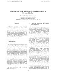
parallel-c<strong>on</strong>necti<strong>on</strong> of H and Q via identifying lt(H)<br />
with lt(Q) and rt(H) with rt(Q), respectively. <str<strong>on</strong>g>The</str<strong>on</strong>g><br />
new terminals of G are lt(G) = lt(H) = lt(Q) and rt(G)<br />
= rt(H) = rt(Q). We denote G = H + Q.<br />
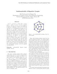
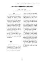
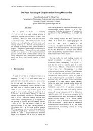
Fig. 1 shows two TTSP graphs H and Q. Fig. 2<br />
and Fig. 3 depict the TTSP graphs = H • Q and<br />
G 2<br />
G 1<br />
= H + Q, respectively.<br />
A linear-time algorithm exists to recognize<br />
whether a graph G is a TTSP graph. A paring tree T<br />
is also generated to illustrate how the graph G is<br />
c<strong>on</strong>structed via series and parallel c<strong>on</strong>necti<strong>on</strong>s [11].<br />
<str<strong>on</strong>g>The</str<strong>on</strong>g> leaves of T corresp<strong>on</strong>d to all edges of G. Since a<br />
general tree can be interpreted as a binary tree easily<br />
[12], this paper <strong>on</strong>ly c<strong>on</strong>siders binary parsing trees.<br />
H<br />
x1<br />
x y<br />
2 1<br />
Figure 1: TTSP graphs H and Q with lt(H) = ,<br />
rt(H) = and lt(Q) = , rt(Q) = y<br />
H<br />
x 1<br />
Q<br />
x2<br />
y1<br />
2<br />
x 2 = y 1<br />
Remarks:<br />
1. G 1 = H • Q.<br />
2. lt(G) = lt(H) = x 1 and rt(G) = rt(Q) = y 2.<br />
G 1<br />
Figure 2: <str<strong>on</strong>g>The</str<strong>on</strong>g> TTSP graph derived by the<br />
series-c<strong>on</strong>necti<strong>on</strong> of H and Q.<br />
H<br />
x 1<br />
y 2<br />
y 2<br />
Q<br />
2. Notati<strong>on</strong>s and Background<br />
x 1 = y 1<br />
x 2 = y 2<br />
<str<strong>on</strong>g>The</str<strong>on</strong>g> class of <strong>Two</strong>-Terminal Series-Parallel<br />
graphs (TTSP graphs) can be defined recursively as<br />
follows [4, 10, 11, 16]: (1) A graph G c<strong>on</strong>sisting of a<br />
single edge e = ( v , v ) is a TTSP graph. v and<br />
v j<br />
i<br />
j<br />
are called the left terminal and the right terminal<br />
of G, respectively. In the rest of this paper, we use<br />
lt(G) and rt(G) to denote the two terminals of G,<br />
respectively, i.e., lt(G) = vi<br />
and rt(G) = v<br />
j<br />
. (2) If H<br />
and Q are two TTSP graphs, then the new graph G<br />
derived by <strong>on</strong>e of the following rules is also a TTSP<br />
graph. (a) G is derived by the series-c<strong>on</strong>necti<strong>on</strong> of H<br />
and Q via identifying rt(H) with lt(Q). <str<strong>on</strong>g>The</str<strong>on</strong>g> new<br />
terminals of G are lt(G) = lt(H) and rt(G) = rt(Q). We<br />
denote G = H • Q. (b) G is derived by the<br />
i<br />
Q<br />
Remarks:<br />
1. G 2 = H + Q.<br />
2. lt(G) = lt(H) = x 1 and rt(G) = rt(H) = x 2.<br />
G 2<br />
Figure 3: <str<strong>on</strong>g>The</str<strong>on</strong>g> TTSP graph derived by the<br />
parallel-c<strong>on</strong>necti<strong>on</strong> of H and Q.<br />
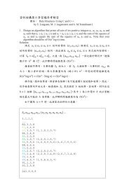
Given a TTSP graph G, let T be its parsing tree<br />
and r is the root of T. For any node z of T, the subtree<br />
rooted at z is denoted by T(z). It is easy to verify that<br />
the subgraph induced by the leaves of T(z) is also a<br />
TTSP graph. So, we use G(z) to denote the subgraph<br />
induced by the leaves of T(z), and V(G(z)) and<br />
E(G(z)) denote its vertex-set and the edge-set,<br />
-355-
<str<strong>on</strong>g>The</str<strong>on</strong>g> 25th Workshop <strong>on</strong> Combinatorial Mathematics and Computati<strong>on</strong> <str<strong>on</strong>g>The</str<strong>on</strong>g>ory<br />
respectively. By this notati<strong>on</strong>, G(r) is just the<br />
original input graph G. In another, each n<strong>on</strong>-leaf<br />
node u of T is associated with a label lb(u). Assume<br />
that q and f are the children of u. If G(u) = G(q) •<br />
G(f), then lb(u) = S and u is called a S-node.<br />
Otherwise, it implies that G(u) = G(q) + G(f). In this<br />
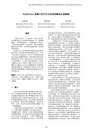
case, lb(u) = P and u is called a P-node. Fig. 4 shows<br />
a TTSP graph G and a corresp<strong>on</strong>ding parsing tree T.<br />
In [19], the authors investigated literatures <strong>on</strong><br />
TTSP graphs for some problems, such as the<br />
minimum feedback vertex problem and the<br />
maximum independent set. Meanwhile, in [8], the<br />
authors shown that APSPL problem <strong>on</strong> planar<br />
graphs with n<strong>on</strong>negative edge-weights can be<br />
2<br />
solved in O( n ) time. But the time-complexity so<strong>on</strong><br />
increases to O(<br />
n<br />
7<br />
3<br />
log( nL)<br />
) if negative<br />
edge-weights are allowed, where L is the absolute<br />
value of the most negative edge-weight. <str<strong>on</strong>g>The</str<strong>on</strong>g> class of<br />
TTSP graphs is an important subclass of planar<br />
graphs. This paper will establish a meaningful<br />
improvement: the WAPSPL problem <strong>on</strong> TTSP<br />
2<br />
graphs can be solved in O( n ) time.<br />
2<br />
3. An O( n )-Time Algorithm<br />
It is so trivial to solve our problem when the input<br />
graph c<strong>on</strong>sists <strong>on</strong>ly a single edge. <str<strong>on</strong>g>The</str<strong>on</strong>g>refore, we<br />
assume that the input graph G c<strong>on</strong>sists of at least two<br />
edges hereafter. To go <strong>on</strong> our discussi<strong>on</strong>, the<br />
following definiti<strong>on</strong>s are introduced firstly.<br />
Definiti<strong>on</strong> 1: For any node z of T(r), the nodes in the<br />
path from z to the root r, except z itself, are called the<br />
ancestors of z.<br />
Definiti<strong>on</strong> 2: For any two distinct vertices<br />
v<br />
j<br />
and<br />
of G(r), the lowest comm<strong>on</strong> ancestor of and<br />
v<br />
j<br />
, denoted as LCA({ vi<br />
, v<br />
j<br />
}) is defined as<br />
follows: (1) If ( vi<br />
, v<br />
j<br />
) is an edge of G(r), then it<br />
implies that ( vi<br />
, v<br />
j<br />
) corresp<strong>on</strong>ds to some leaf node<br />
z and LCA({ vi<br />
, v<br />
j<br />
}) is defined to be z itself. (2) If<br />
( v , v ) is not an edge of G(r), then there must<br />
i<br />
j<br />
exist two leaf nodes p and q such that<br />
v i<br />
vi<br />
is the <strong>on</strong>e<br />
vertex of the edge corresp<strong>on</strong>ding to p and is the<br />
<strong>on</strong>e vertex of the edge corresp<strong>on</strong>ding to q. In this<br />
situati<strong>on</strong>, LCA({ vi<br />
, v<br />
j<br />
}) is defined to be the node<br />
u farthest from r such that u is a ancestor of both p<br />
and q.<br />
v i<br />
v j<br />
S<br />
<br />
(v 1, v 3)<br />
S<br />
<br />
v 1<br />
P<br />
<br />
v 2<br />
(v 6, v 7) (v 1, v 4)<br />
v 3<br />
v 4<br />
S<br />
<br />
P<br />
<br />
(v 7, v 8)<br />
S<br />
<br />
v 6<br />
v 5<br />
v 8<br />
v 7<br />
(v 1, v 2)<br />
S<br />
<br />
(v 4, v 7) (v 2, v 5)<br />
S<br />
<br />
(v 5, v 8)<br />
P<br />
<br />
(v 3, v 6)<br />
Remarks:<br />
For each n<strong>on</strong>-leaf node u, denotes the terminals of G(u).<br />
Figure 4: A TTSP graph G and its corresp<strong>on</strong>ding<br />
parsing tree T.<br />
Definiti<strong>on</strong> 3: Suppose that u is a P-node of T(r). u is<br />
called a bottom P-node if all nodes of T(u) are either<br />
S-nodes or leaf nodes, except u itself. Otherwise, u is<br />
called a n<strong>on</strong>-bottom P-node. In additi<strong>on</strong>, u is called a<br />
top P-node if the ancestors of u in T(r) are all<br />
S-nodes. If u is not a top P-node, then u is called a<br />
n<strong>on</strong>-top P-node. By this definiti<strong>on</strong>, u can be a top<br />
P-node and a bottom P-node at the same time.<br />
Definiti<strong>on</strong> 4: For any bottom P-node u of T(r),<br />
pair_set(u) is defined as {{ vi<br />
, v<br />
j<br />
} | vi<br />
, v<br />
j<br />
∈<br />
V(G(u))}<br />
Definiti<strong>on</strong> 5: For any n<strong>on</strong>-bottom P-node u of T(r),<br />
pair_set(u) is defined as {{ vi<br />
, v<br />
j<br />
} | vi<br />
, v<br />
j<br />
∈<br />
V(G(u))} – ∪<br />
pair_set( v)<br />
.<br />
for all P-node<br />
v≠u<br />
of T ( u)<br />
Definiti<strong>on</strong> 6: For each n<strong>on</strong>-top P-node u, the lowest<br />
P-node ancestor of u, denoted as LPNA(u) is the<br />
P-node f satisfying the following c<strong>on</strong>diti<strong>on</strong>s: (1) f is<br />
nearest to u, and (2) f is in the path from u to the root<br />
r.<br />
Definiti<strong>on</strong> 7: For each n<strong>on</strong>-leaf node z of T(r), let q<br />
and f be the left child and the right child of z,<br />
respectively. Define left_descendants(z) = {x | x is a<br />
node in T(q).} and right_descendants(z) = {x | x is a<br />
node in T(f).}<br />
<str<strong>on</strong>g>The</str<strong>on</strong>g> following lemma can be easily established.<br />
Lemma 1: For any two distinct vertices vi<br />
, v<br />
j<br />
of<br />
G(r), there exists at most <strong>on</strong>e P-node u such that<br />
(v 2, v 8)<br />
-356-
<str<strong>on</strong>g>The</str<strong>on</strong>g> 25th Workshop <strong>on</strong> Combinatorial Mathematics and Computati<strong>on</strong> <str<strong>on</strong>g>The</str<strong>on</strong>g>ory<br />
{ v , v } ∈ pair_set(u). If no P-node u such that<br />
i<br />
j<br />
pair_set(u) c<strong>on</strong>tains { v , v }, then LCA({ v ,<br />
v j<br />
i<br />
}) must be either a leaf node or a S-node, and all<br />
ancestors of LCA({ v , v }) must also be S-nodes.<br />
i<br />
Otherwise, the <strong>on</strong>ly P-node c<strong>on</strong>taining { v , v }<br />
will be denoted as PN({ v , v }). Meanwhile,<br />
pair_set(u) for all P-nodes u can be computed in<br />
2<br />
O( n ) time.<br />
j<br />
Since our objective is to compute Len( v ⇒ v )<br />
and Len( v ⇒ v ), for all distinct vertices v and<br />
v j<br />
j<br />
of G(r), <str<strong>on</strong>g>The</str<strong>on</strong>g> following reas<strong>on</strong>ing can then be<br />
made based <strong>on</strong> Lemma 1.<br />
i<br />
Definiti<strong>on</strong> 8: For any two distinct vertices vi<br />
, v<br />
j<br />
of G(r), if no P-node u such that pair_set(u) c<strong>on</strong>tains<br />
{ vi<br />
, v<br />
j<br />
}, then the pair { vi<br />
, v<br />
j<br />
} is called a Type I<br />
pair. Otherwise, there exists <strong>on</strong>ly <strong>on</strong>e P-node u such<br />
that { vi<br />
, v<br />
j<br />
} ∈ pair_set(u) and the pair { vi<br />
, v<br />
j<br />
}<br />
is called a Type II pair.<br />
Lemma 2: For any two distinct vertices vi<br />
, v<br />
j<br />
of<br />
G(r), { vi<br />
, v<br />
j<br />
} is either a Type I pair or a Type II<br />
pair.<br />
Definiti<strong>on</strong> 9: For any node z of T(r) and any two<br />
distinct vertices v and v of G(z), define<br />
to<br />
i<br />
( )<br />
Len z ( v ⇒ v ) = min{Len(P) | P is a path from<br />
vi<br />
v<br />
j<br />
i<br />
j<br />
i<br />
j<br />
c<strong>on</strong>sisting of the edges <strong>on</strong>ly in E(G(z)).}<br />
( )<br />
and Len z ( v<br />
j<br />
⇒ vi<br />
) = min{Len(P) | P is a path<br />
from v<br />
j<br />
to vi<br />
c<strong>on</strong>sisting of the edges <strong>on</strong>ly in<br />
E(G(z)).}<br />
Definiti<strong>on</strong> 10: For any P-node u of T(r) and any two<br />
distinct vertices vi<br />
and v<br />
j<br />
of G(u), define<br />
OutLen( vi<br />
⇒ v<br />
j<br />
) = min{Len(P) | P is a path from<br />
vi<br />
to v<br />
j<br />
c<strong>on</strong>sisting of the edges <strong>on</strong>ly in E –<br />
E(G(u)).} and OutLen( v<br />
j<br />
⇒ vi<br />
) = min{Len(P) | P<br />
is a path from v to v c<strong>on</strong>sisting of the edges <strong>on</strong>ly<br />
j<br />
i<br />
in E – E(G(u)).} If there exists no path from<br />
v j<br />
c<strong>on</strong>sisting of the edges <strong>on</strong>ly in E – E(G(u)), then<br />
j<br />
j<br />
i<br />
i<br />
i<br />
v i<br />
i<br />
j<br />
j<br />
to<br />
set OutLen( v ⇒ v ) = ∞. Also, if there exists no<br />
i<br />
j<br />
path from v to v c<strong>on</strong>sisting of the edges <strong>on</strong>ly in<br />
j<br />
i<br />
E – E(G(u)), then set OutLen( v ⇒ v ) = ∞.<br />
Lemma 3: For any type I pair { v , v } of G(r), let<br />
u = LCA({ v , v }). We must have Len( v ⇒ v )<br />
i<br />
( )<br />
= Len u ( v ⇒ v ) and Len( v ⇒ v ) =<br />
( )<br />
Len u<br />
( v ⇒ v ).<br />
j<br />
i<br />
j<br />
i<br />
j<br />
[1] [2] [α]<br />
Proof: Let u--u<br />
--u<br />
--…-- u = r be the path<br />
[1] [2]<br />
from u to r in T(r). It implies that u , u , …,<br />
[α]<br />
u are the ancestors of u and they must be all<br />
S-nodes. By the definiti<strong>on</strong>s of TTSP graphs and their<br />
parsing trees, G(r) must be c<strong>on</strong>structed via<br />
[1] [2]<br />
series-c<strong>on</strong>necti<strong>on</strong>s marked at lb( u ), lb( u ), …,<br />
[α]<br />
lb( u ), respectively. It is easy to verify that<br />
( )<br />
Len( v ⇒ v ) = Len u ( v ⇒ v ) and Len( v<br />
i<br />
j<br />
( )<br />
⇒ ) = Len u ( v ⇒ v ). <br />
v i<br />
j<br />
Lemma 4: For any type II pair { v , v } of G(r), let<br />
u = PN({ v , v }). In additi<strong>on</strong>, let z = LPNA(u) and<br />
v<br />
s<br />
i<br />
= lt(G(u)) and v = rt(G(u)). <str<strong>on</strong>g>The</str<strong>on</strong>g>n, we have the<br />
following formulas.<br />
Len( v ⇒ v )<br />
i<br />
i<br />
j<br />
j<br />
( )<br />
= min{ Len u ( v ⇒ v ),<br />
t<br />
i<br />
j<br />
i<br />
( )<br />
Len a ( vi<br />
⇒ vs<br />
) + OutLen( vs<br />
⇒ vt<br />
)<br />
( )<br />
+ Len b ( v ⇒ v ),<br />
t<br />
j<br />
( )<br />
Len a ( vi<br />
⇒ vt<br />
) + OutLen( vt<br />
⇒ vs<br />
)<br />
( )<br />
+ Len b ( v ⇒ v )}<br />
Len( v ⇒ v )<br />
j<br />
i<br />
( )<br />
= min{ Len u ( v ⇒ v ),<br />
j<br />
s<br />
i<br />
j<br />
( )<br />
Len b ( v<br />
j<br />
⇒ vs<br />
) + OutLen( vs<br />
⇒ vt<br />
)<br />
( )<br />
+ Len a ( v ⇒ v ),<br />
t i<br />
( )<br />
Len b ( v<br />
j<br />
⇒ vt<br />
) + OutLen( vt<br />
⇒ vs<br />
)<br />
( )<br />
+ Len a ( v ⇒ v )}<br />
s<br />
Proof: Since Len( v ⇒ v ) and Len( v ⇒ v )<br />
are just symmetrical by interchanging the roles of<br />
v and v . We just show the correctness of the<br />
i<br />
j<br />
i<br />
j<br />
i<br />
j<br />
i<br />
i<br />
j<br />
j<br />
j<br />
i<br />
j<br />
i<br />
i<br />
i<br />
j<br />
j<br />
j<br />
-357-
<str<strong>on</strong>g>The</str<strong>on</strong>g> 25th Workshop <strong>on</strong> Combinatorial Mathematics and Computati<strong>on</strong> <str<strong>on</strong>g>The</str<strong>on</strong>g>ory<br />
formula about Len( v ⇒ v ). <str<strong>on</strong>g>The</str<strong>on</strong>g> following cases<br />
i<br />
are c<strong>on</strong>sidered, respectively.<br />
Case 1. u is a top P-node<br />
It is easy to ascertain OutLen( v ⇒ v ) =<br />
OutLen( v ⇒ v ) = ∞, i.e., each path P from v to<br />
v j<br />
t<br />
s<br />
c<strong>on</strong>sists of <strong>on</strong>ly edges in E(G(u)). Thus, the<br />
formula holds for this case.<br />
Case 2. u is a n<strong>on</strong>-top P-node<br />
In this case, at least <strong>on</strong>e ancestor of u is also a<br />
P-node. By the c<strong>on</strong>structi<strong>on</strong> rules of TTSP graphs,<br />
at least <strong>on</strong>e path from vs<br />
to vt<br />
c<strong>on</strong>sists of the<br />
edges <strong>on</strong>ly in E – E(G(u)) and at least <strong>on</strong>e path from<br />
vt<br />
to vs<br />
c<strong>on</strong>sists of the edges <strong>on</strong>ly in E – E(G(u)).<br />
<str<strong>on</strong>g>The</str<strong>on</strong>g>refore, it is easy to verify that the formula holds.<br />
<br />
Based up<strong>on</strong> all reas<strong>on</strong>ing so far, the following<br />
algorithm can solve the WAPSPL <strong>on</strong> TTSP graphs<br />
correctly.<br />
Algorithm WAPSPL_TTSP<br />
Input: A weighted TTSP graph G and its<br />
corresp<strong>on</strong>ding parsing tree T(r) such that<br />
pair_set(u),<br />
left_descendants(u),<br />
right_descendants(u), and LPAN(u), for all<br />
P-nodes u, have been computed.<br />
/* We assume that the vertices of G(r) are<br />
v1<br />
, …, vn<br />
. */<br />
Output: <str<strong>on</strong>g>The</str<strong>on</strong>g> array L[1 … n, 1 … n] such that L[i, j]<br />
= Len( v ⇒ v ) and L[j, i] = Len( v ⇒<br />
v i<br />
i<br />
j<br />
j<br />
), for all 1 ≤ i, j ≤ n.<br />
/* <str<strong>on</strong>g>The</str<strong>on</strong>g> array L is global to all phases of the<br />
algorithm. */<br />
Phase I:<br />
L[i, j] = [i, j] = L [i, j] = 0, 1 ≤ i ≤ n, 1 ≤ j ≤ n;<br />
L1<br />
2<br />
for each P-node u of T(r)<br />
Compute L 1<br />
(rt(G(u)) ⇒ lt(G(u))),<br />
L2<br />
(rt(G(u)) ⇒ lt(G(u))), L1<br />
(lt(G(u)) ⇒<br />
rt(G(u))), and L 2<br />
(lt(G(u)) ⇒ rt(G(u)));<br />
( )<br />
Len u (rt(G(u)) ⇒ lt(G(u))) =<br />
min{ L1<br />
(rt(G(u)) ⇒ lt(G(u))), L2<br />
(rt(G(u)) ⇒<br />
lt(G(u)))};<br />
( )<br />
Len u (lt(G(u)) ⇒ rt(G(u))) =<br />
min{ L 1<br />
(lt(G(u)) ⇒ rt(G(u))), and<br />
L 2<br />
(lt(G(u)) ⇒ rt(G(u)))};<br />
endfor<br />
s<br />
t<br />
j<br />
i<br />
for each S-node z of T(r)<br />
( )<br />
Compute Len z ( v ⇒ v ) and<br />
( )<br />
Len z ( v<br />
j<br />
⇒ vi<br />
), for all vi<br />
and v<br />
j<br />
of G(z);<br />
endfor<br />
/* For simplicity, we use two two-dimensi<strong>on</strong>al<br />
arrays L1<br />
[1 … n, 1 … n] and L2<br />
[1 … n, 1 … n]<br />
to store L1<br />
( vs<br />
⇒ vt<br />
), L2<br />
( vs<br />
⇒ vt<br />
), L1<br />
( vt<br />
⇒ vs<br />
), and L2<br />
( vt<br />
⇒ vs<br />
), for all vs<br />
and vt<br />
such that < vs<br />
, vt<br />
> are terminals of some P-node<br />
u.. Meanwhile, these two arrays are global to all<br />
phases of the algorithm. */<br />
Phase II:<br />
for each P-node u of T(r)<br />
Compute OutLen(rt(G(u)) ⇒ lt(G(u))) and<br />
OutLen(lt(G(u)) ⇒ rt(G(u)));<br />
endfor<br />
/* If there is no P-node in T(r), then this phase<br />
does nothing. */<br />
/* For simplicity, we also use a two-dimensi<strong>on</strong>al<br />
array OL[1 … n, 1 … n] to store OutLen( v s<br />
⇒<br />
vt<br />
) and OutLen( vt<br />
⇒ vs<br />
), for all vs<br />
and vt<br />
such that < vs<br />
, vt<br />
> are terminals of some P-node<br />
u. Meanwhile, OL[i, j] is initialized to be ∞, for<br />
all 1 ≤ i, j ≤ n. and this array is global to all phases<br />
of the algorithm. */<br />
Phase III:<br />
for each P-node u of T(r)<br />
for each pair { vi<br />
, v<br />
j<br />
} in pair_set(u)<br />
Use the arrays OL, L1<br />
, and L2<br />
to adjust<br />
L[i, j] for obtaining Len( vi<br />
⇒ v<br />
j<br />
);<br />
endfor<br />
endfor<br />
End WAPSPL_TTSP<br />
3.1 Phase I<br />
For each node z of T(r), let lt(G(z)) =<br />
v j<br />
i<br />
j<br />
and<br />
rt(G(z)) = . <str<strong>on</strong>g>The</str<strong>on</strong>g> following cases should be<br />
c<strong>on</strong>sidered.<br />
Case 1. z is a leaf node<br />
In this case, we just let L[i, j] = W( vi<br />
→ v<br />
j<br />
) and<br />
L[j, i] = W( v<br />
j<br />
→ vi<br />
).<br />
Case 2. z is a S-Node<br />
Let q and f be the left child and the right child of z,<br />
respectively, i.e., G(z) = G(q) • G(f). In additi<strong>on</strong>, let<br />
v i<br />
-358-
<str<strong>on</strong>g>The</str<strong>on</strong>g> 25th Workshop <strong>on</strong> Combinatorial Mathematics and Computati<strong>on</strong> <str<strong>on</strong>g>The</str<strong>on</strong>g>ory<br />
v = lt(G(q)) and v = rt(G(q)); and let v =<br />
i<br />
lt(G(f)) and<br />
v j<br />
be performed.<br />
k<br />
= rt(G(f)). <str<strong>on</strong>g>The</str<strong>on</strong>g> following codes will<br />
recursively compute L[s, t], and L[t, s], for ,<br />
v t<br />
∈ V(G(q));<br />
recursively compute L[s, t], and L[t, s], for ,<br />
v t<br />
∈ V(G(f));<br />
L[i, j] = L[i, k] + L[k, j];<br />
L[j, i] = L[j, k] + L[k, i];<br />
for each pair of vertices v ≠ v such that v ∈<br />
V(G(q)) – { v , v } and v ∈ V(G(f)) – { v ,<br />
v j<br />
}<br />
i<br />
k<br />
/* If <strong>on</strong>e of V(G(q)) – { v , v } and V(G(f)) –<br />
{ v , v } is empty, then we just skip this loop. */<br />
k<br />
j<br />
L[a, b] = L[a, k] + L[k, b];<br />
L[b, a] = L[b, k] + L[k, a];<br />
endfor<br />
vi<br />
∈ V(G(f)) – { vk<br />
, v<br />
j<br />
}<br />
v v<br />
for each pair of vertices and v such that<br />
a<br />
i<br />
b<br />
k<br />
b<br />
b<br />
k<br />
v s<br />
v s<br />
a<br />
k<br />
vb<br />
/* If V(G(f)) – {<br />
k<br />
,<br />
j<br />
} is empty, then we just<br />
skip this loop. */<br />
L[i, b] = L[i, k] + L[k, b];<br />
L[b, i] = L[b, k] + L[k, i];<br />
endfor<br />
for each pair of vertices v and v such that<br />
∈ V(G(q)) – { vi<br />
, vk<br />
}<br />
/* If V(G(q)) – { vi<br />
, vk<br />
} is empty, then we just<br />
skip this loop. */<br />
L[a, j] = L[a, k] + L[k, j];<br />
L[j, a] = L[j, k] + L[k, a];<br />
endfor<br />
a<br />
j<br />
va<br />
Case 3. z is a P-node<br />
Let q and f be the left child and the right child of z,<br />
respectively, i.e., G(z) = G(q) + G(f). In this case,<br />
lt(G(q)) = lt(G(f)) = vi<br />
and rt(G(q)) = lt(G(f)) = v<br />
j<br />
.<br />
<str<strong>on</strong>g>The</str<strong>on</strong>g> following codes will be performed.<br />
recursively compute L[s, t], and L[t, s], for ,<br />
v t<br />
∈ V(G(q));<br />
L<br />
1<br />
[i, j] = L[i, j];<br />
[j, i] = L[j, i];<br />
L 1<br />
recursively compute L[s, t], and L[t, s], for ,<br />
v t<br />
∈ V(G(f));<br />
L<br />
2<br />
[i, j] = L[i, j];<br />
L 2<br />
[j, i] = L[j, i];<br />
v s<br />
v s<br />
L[i, j] = min{ L1<br />
[i, j], L2<br />
[i, j]};<br />
L[j, i] = min{ [j, i], L [j, i]};<br />
L1<br />
2<br />
2<br />
Lemma 5: Phase I can be d<strong>on</strong>e in O( n ) time.<br />
Proof: To complete Phase I, each pair of vertices<br />
v j<br />
and is examined c<strong>on</strong>stant times and each node of<br />
T(r) is also examined c<strong>on</strong>stant times. This implies<br />
2<br />
that Phase I can be d<strong>on</strong>e in O( n ) time. <br />
3.2 Phase II<br />
It is easy to see that LPNA(u), for each P-node u,<br />
can be obtained by the post-order traversal <strong>on</strong> T and<br />
the time-complexity is linear. Based <strong>on</strong> the<br />
reas<strong>on</strong>ing and the results of so far, Phase II can be<br />
achieved by breadth-first traversal <strong>on</strong> T from the<br />
root r. For each n<strong>on</strong>-top P-node u, assume that f =<br />
LPNA(u) and the terminals of G(u) and G(f) are<br />
< vi<br />
, v<br />
j<br />
> and < vs<br />
, vt<br />
>, respectively. <str<strong>on</strong>g>The</str<strong>on</strong>g><br />
following code will be performed.<br />
if (u ∈ left_descendants(f))<br />
OL[i, j] = L[i, s] + [s, t] + L[t, j];<br />
L 2<br />
L 2<br />
OL[j, i] = L[j, t] + [t, s] + L[s, i];<br />
else /* u ∈ right_descendants(f). */<br />
OL[i, j] = L[i, s] + [s, t] + L[t, j];<br />
OL[j, i] = L[j, t] +<br />
endif<br />
L 1<br />
[t, s] + L[s, i];<br />
L 1<br />
<str<strong>on</strong>g>The</str<strong>on</strong>g> following lemma can be verified easily.<br />
2<br />
Lemma 6: Phase II can be d<strong>on</strong>e in O( n )-time.<br />
3.3 Phase III<br />
This phase will be achieved by depth-first<br />
traversal <strong>on</strong> T from the root r. For each P-node u, let<br />
q and f be the left child and the right child of u,<br />
respectively, i.e., G(u) = G(q) + G(f). In this case,<br />
lt(G(q)) = lt(G(f)) = vi<br />
and rt(G(q)) = lt(G(f)) = v<br />
j<br />
.<br />
<str<strong>on</strong>g>The</str<strong>on</strong>g> following codes will be performed.<br />
for each pair { va<br />
, vb<br />
} ∈ pair_set(u)<br />
docase<br />
case va<br />
, vb<br />
∈ V(G(q))<br />
L[a, b] = min{L[a, b],<br />
L[a, i] + L 2<br />
[i, j] + L[j, b],<br />
L[a, j] + L 2<br />
[j, i] + L[i, b],<br />
L[a, i] + OL[i, j] + L[j, b],<br />
L[a, j] + OL[j, i] + L[i, b]};<br />
L[b, a] = min{L[a, b], L[b, i] + L 2<br />
[i, j]<br />
v i<br />
-359-
<str<strong>on</strong>g>The</str<strong>on</strong>g> 25th Workshop <strong>on</strong> Combinatorial Mathematics and Computati<strong>on</strong> <str<strong>on</strong>g>The</str<strong>on</strong>g>ory<br />
L 2<br />
+ L[j, a], L[b, j] + [j, i] + L[i, a],<br />
L[b, i] + OL[i, j] + L[j, a], L[b, j] +<br />
OL[j, i] + L[i, a]};<br />
break;<br />
case v , v ∈ V(G(f))<br />
a<br />
b<br />
L[a, b] = min{L[a, b],<br />
L[a, i] + [i, j] + L[j, b],<br />
L 1<br />
L[a, j] + L 1<br />
[j, i] + L[i, b],<br />
L[a, i] + OL[i, j] + L[j, b],<br />
L[a, j] + OL[j, i] + L[i, b]};<br />
L[b, a] = min{L[a, b], L[b, i] + [i, j] + L[j,<br />
L 1<br />
L 1<br />
a], L[b, j] + [j, i] + L[i, a], L[b, i] +<br />
OL[i, j] + L[j, a], L[b, j] + OL[j, i] +<br />
L[i, a]};<br />
break;<br />
case ( v ∈ V(G(q)) and v ∈ V(G(f))) or ( v ∈<br />
a<br />
V(G(f)) and<br />
v b<br />
b<br />
∈ V(G(q)))<br />
L[a, b] = min{L[a, i] + L[i, b],<br />
L[a, j] + L[j, b],<br />
L[a, i] + OL[i, j] + L[j, b],<br />
L[a, j] + OL[j, i] + L[i, b]};<br />
L[b, a] = min{L[b, i] + L[i, a],<br />
L[b, j] + L[j, a],<br />
L[b, i] + OL[i, j] + L[j, a],<br />
L[b, j] + OL[j, i] + L[i, a]};<br />
break;<br />
endcase<br />
endfor<br />
2<br />
Lemma 7: Phase III can be d<strong>on</strong>e in O( n )-time.<br />
<str<strong>on</strong>g>All</str<strong>on</strong>g> reas<strong>on</strong>ing and results so far can easily imply<br />
the following theorem.<br />
<str<strong>on</strong>g>The</str<strong>on</strong>g>orem 1: <str<strong>on</strong>g>The</str<strong>on</strong>g> weighted APSPL problem <strong>on</strong><br />
2<br />
TTSP graphs can be solved in O( n ) time.<br />
4. C<strong>on</strong>clusi<strong>on</strong>s<br />
In [8], the authors shown that APSPL problem <strong>on</strong><br />
planar graphs with n<strong>on</strong>negative edge-weights can be<br />
2<br />
solved in O( n ) time. But the time-complexity so<strong>on</strong><br />
7<br />
3<br />
increases to O( n log( nL)<br />
) if negative<br />
edge-weights are allowed, where L is the absolute<br />
value of the most negative edge-weight. <str<strong>on</strong>g>The</str<strong>on</strong>g> class of<br />
TTSP graphs is a vital subclass of the class of planar<br />
graphs. This paper has established a meaningful<br />
improvement: the WAPSPL problem <strong>on</strong> TTSP<br />
2<br />
graphs can be solved in O( n ) time. Our algorithm<br />
a<br />
⎛n⎞<br />
is time-optimal in worst case since there are ⎜ ⎟ =<br />
⎝ 2⎠<br />
2<br />
O( n ) pairs of distinct vertices in any graph G.<br />
In the future, it is very important and worthy to<br />
extend our result to the classes of graphs with the<br />
property m = O(n), such as planar graphs. In another,<br />
studying the WAPSPL <strong>on</strong> other classes of graphs<br />
such as bipartite graphs, permutati<strong>on</strong> graphs, is also<br />
a practical and interesting issue.<br />
References<br />
[1] P. D’ Alberto and A. Nicolau, “R-Kleene: A<br />
High-Performance Divide-and-C<strong>on</strong>quer<br />
Algorithm for the <str<strong>on</strong>g>All</str<strong>on</strong>g>-Pair <str<strong>on</strong>g>Shortest</str<strong>on</strong>g> <str<strong>on</strong>g>Path</str<strong>on</strong>g> for<br />
Densely C<strong>on</strong>nected Networks”, Algorithmica,<br />
Vol. 47, pp. 203-213, 2007.<br />
[2] E. Cohen, “Polylog-Time and Near-Linear<br />
Work Approximati<strong>on</strong> Scheme for Undirected<br />
<str<strong>on</strong>g>Shortest</str<strong>on</strong>g> <str<strong>on</strong>g>Path</str<strong>on</strong>g>s”, Journal of the ACM, Vol. 47,<br />
No. 1, January 2000.<br />
[3] E. W. Dijkstra, “A Note <strong>on</strong> <strong>Two</strong> <str<strong>on</strong>g>Problem</str<strong>on</strong>g>s in<br />
C<strong>on</strong>nexi<strong>on</strong> with Graphs”, Numerische<br />
Mathematik, Vol. 1, pp. 269-271, 1959.<br />
[4] R. J. Duffin, “Topology of Series-Parallel<br />
Networks”, J. Math., Appl. 10, pp. 303-318,<br />
1965.<br />
[5] M. L. Fredman and R. E. Tarjan, “Fib<strong>on</strong>acci<br />
Heaps and <str<strong>on</strong>g>The</str<strong>on</strong>g>ir Uses in Improved Network<br />
Optimizati<strong>on</strong> Algorithms”, Journal of ACM,<br />
Vol. 34, pp. 596-615, 1987.<br />
[6] M. L. Fredman and D. E. Willard,<br />
“Trans-dichotomous Algorithms for Minimum<br />
Spanning Trees and <str<strong>on</strong>g>Shortest</str<strong>on</strong>g> <str<strong>on</strong>g>Path</str<strong>on</strong>g>s”, Journal of<br />
Computer and System Sciences, Vol. 48, pp.<br />
533-551, 1994.<br />
[7] Y. Han, “Improved Algorithm for <str<strong>on</strong>g>All</str<strong>on</strong>g> <str<strong>on</strong>g>Pairs</str<strong>on</strong>g><br />
<str<strong>on</strong>g>Shortest</str<strong>on</strong>g> <str<strong>on</strong>g>Path</str<strong>on</strong>g>s”, Informati<strong>on</strong> Processing<br />
Letters, Vol. 91, pp. 245-250, 2004.<br />
[8] M. R. Henzinger, P. Klein, S. Rao, and S.<br />
Subramanian, “Faster <str<strong>on</strong>g>Shortest</str<strong>on</strong>g>-<str<strong>on</strong>g>Path</str<strong>on</strong>g><br />
Algorithms for Planar Graphs”, Journal of<br />
Computer and System Sciences, Vol. 55, Iss. 1,<br />
pp. 3-23, 1997.<br />
[9] C-W Ho and J-M Chang, “Solving <str<strong>on</strong>g>The</str<strong>on</strong>g><br />
<str<strong>on</strong>g>All</str<strong>on</strong>g>-pairs-shortest-length <str<strong>on</strong>g>Problem</str<strong>on</strong>g> <strong>on</strong> Chordal<br />
Bipartite Graphs”, Informati<strong>on</strong> Processing<br />
Letters, Vol. 69, pp. 87-93, 1999.<br />
[10] R. H. Jan, L. H. Hsu, and Y. Y. Lee, “<str<strong>on</strong>g>The</str<strong>on</strong>g><br />
Most Vital Edges with Respect to the Number<br />
of Spanning Trees in <strong>Two</strong>-Terminal<br />
Series-Parallel Graphs”, Bit, Vol. 32, pp.<br />
403-412, 1992.<br />
[11] T. Kikuno, N. Yoshida, and Y. Kakuda, “A<br />
Linear Algorithm for the Dominati<strong>on</strong> Number<br />
-360-
of a Series-Parallel Graph”, Discrete Applied<br />
Mathematics, Vol. 5, pp. 299-311, 1983.<br />
[12] D. E. Knuth, <str<strong>on</strong>g>The</str<strong>on</strong>g> Art of Computer<br />
Programming, Vol. 1, Fundamental<br />
Algorithms, Addis<strong>on</strong>-Wesley, 1968.<br />
2<br />
[13] P. Mirchandani, “A Simple O( n ) Algorithm<br />
for the <str<strong>on</strong>g>All</str<strong>on</strong>g>-<str<strong>on</strong>g>Pairs</str<strong>on</strong>g> <str<strong>on</strong>g>Shortest</str<strong>on</strong>g> <str<strong>on</strong>g>Path</str<strong>on</strong>g> <str<strong>on</strong>g>Problem</str<strong>on</strong>g> <strong>on</strong> an<br />
Interval Graph”, Networks, Vol. 27, pp.<br />
215-217, 1996.<br />
[14] S. Pettie, “A Faster <str<strong>on</strong>g>All</str<strong>on</strong>g>-<str<strong>on</strong>g>Pairs</str<strong>on</strong>g> <str<strong>on</strong>g>Shortest</str<strong>on</strong>g> <str<strong>on</strong>g>Path</str<strong>on</strong>g><br />
Algorithm for Real-<str<strong>on</strong>g>Weighted</str<strong>on</strong>g> Sparse Graphs”,<br />
Lecture Notes in Computer Science, Vol. 2380,<br />
pp. 85-97, 2002.<br />
[15] R. Ravi, M. V. Marathe, and C. P. Rangan, “An<br />
Optimal Algorithm to Solve the <str<strong>on</strong>g>All</str<strong>on</strong>g>-Pair<br />
<str<strong>on</strong>g>Shortest</str<strong>on</strong>g> <str<strong>on</strong>g>Path</str<strong>on</strong>g> <str<strong>on</strong>g>Problem</str<strong>on</strong>g> <strong>on</strong> Interval Graphs”,<br />
Networks, Vol. 22, pp. 21-35, 1992.<br />
[16] K. Takamizwa, T. Nishizeki, and N. Saito,<br />
“Linear-Time Computability of<br />
Combinatorial <str<strong>on</strong>g>Problem</str<strong>on</strong>g>s <strong>on</strong> Series-Parallel<br />
Graphs”, Journal of the A.C.M., Vol. 29, No.<br />
3, pp. 623-641, 1982.<br />
3<br />
[17] T. Takaoka, “An O( n loglogn / logn) Time<br />
Algorithm for the <str<strong>on</strong>g>All</str<strong>on</strong>g>-<str<strong>on</strong>g>Pairs</str<strong>on</strong>g> <str<strong>on</strong>g>Shortest</str<strong>on</strong>g> <str<strong>on</strong>g>Path</str<strong>on</strong>g><br />
<str<strong>on</strong>g>Problem</str<strong>on</strong>g>”, Informati<strong>on</strong> Processing Letters.,<br />
Vol. 96, pp. 155-161, 2005.<br />
[18] M. Thorup, “Undirected Single-Source<br />
<str<strong>on</strong>g>Shortest</str<strong>on</strong>g> <str<strong>on</strong>g>Path</str<strong>on</strong>g>s with Positive Integer Weights in<br />
Linear Time, Journal of the ACM, Vol. 1l, No.<br />
1, 1999.<br />
[19] C-KYen and C-Y Tang, A Study <strong>on</strong> the<br />
Searchlight Guarding <str<strong>on</strong>g>Problem</str<strong>on</strong>g>, Ph.D.<br />
Dissertati<strong>on</strong>, Department of Computer<br />
Science, Nati<strong>on</strong>al Tsing Hua University,<br />
1996.<br />
<str<strong>on</strong>g>The</str<strong>on</strong>g> 25th Workshop <strong>on</strong> Combinatorial Mathematics and Computati<strong>on</strong> <str<strong>on</strong>g>The</str<strong>on</strong>g>ory<br />
-361-