Observables and Measurements in Quantum Mechanics
Observables and Measurements in Quantum Mechanics
Observables and Measurements in Quantum Mechanics

Create successful ePaper yourself
Turn your PDF publications into a flip-book with our unique Google optimized e-Paper software.
Chapter 13<br />
<strong>Observables</strong> <strong>and</strong> <strong>Measurements</strong> <strong>in</strong> <strong>Quantum</strong><br />
<strong>Mechanics</strong><br />
Till now, almost all attention has been focussed on discuss<strong>in</strong>g the state of a quantum system.<br />
As we have seen, this is most succ<strong>in</strong>ctly done by treat<strong>in</strong>g the package of <strong>in</strong>formation that<br />
def<strong>in</strong>es a state as if it were a vector <strong>in</strong> an abstract Hilbert space. Do<strong>in</strong>g so provides the mathematical<br />
mach<strong>in</strong>ery that is needed to capture the physically observed properties of quantum systems.<br />
A method by which the state space of a physical system can be set up was described <strong>in</strong> Section<br />
8.4.2 where<strong>in</strong> an essential step was to associate a set of basis states of the system with the exhaustive<br />
collection of results obta<strong>in</strong>ed when measur<strong>in</strong>g some physical property, or observable, of<br />
the system. This l<strong>in</strong>k<strong>in</strong>g of particular states with particular measured results provides a way that<br />
the observable properties of a quantum system can be described <strong>in</strong> quantum mechanics, that is <strong>in</strong><br />
terms of Hermitean operators. It is the way <strong>in</strong> which this is done that is the ma<strong>in</strong> subject of this<br />
Chapter.<br />
13.1 <strong>Measurements</strong> <strong>in</strong> <strong>Quantum</strong> <strong>Mechanics</strong><br />
One of the most difficult <strong>and</strong> controversial problems<br />
<strong>in</strong> quantum mechanics is the so-called measurement<br />
problem. Op<strong>in</strong>ions on the significance of this problem<br />
vary widely. At one extreme the attitude is that<br />
there is <strong>in</strong> fact no problem at all, while at the other<br />
extreme the view is that the measurement problem<br />
is one of the great unsolved puzzles of quantum mechanics.<br />
The issue is that quantum mechanics only<br />
provides probabilities for the different possible outcomes<br />
<strong>in</strong> an experiment – it provides no mechanism<br />
by which the actual, f<strong>in</strong>ally observed result, comes<br />
about. Of course, probabilistic outcomes feature <strong>in</strong><br />
many areas of classical physics as well, but <strong>in</strong> that<br />
case, probability enters the picture simply because<br />
there is <strong>in</strong>sufficient <strong>in</strong>formation to make a def<strong>in</strong>ite<br />
prediction. In pr<strong>in</strong>ciple, that miss<strong>in</strong>g <strong>in</strong>formation is<br />
<strong>Quantum</strong><br />
System S<br />
Measur<strong>in</strong>g<br />
Apparatus<br />
M<br />
Surround<strong>in</strong>g Environment E<br />
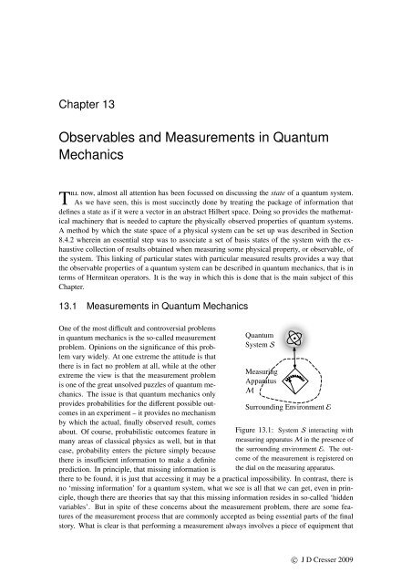
Figure 13.1: System S <strong>in</strong>teract<strong>in</strong>g with<br />
measur<strong>in</strong>g apparatus M <strong>in</strong> the presence of<br />
the surround<strong>in</strong>g environment E. The outcome<br />
of the measurement is registered on<br />
the dial on the measur<strong>in</strong>g apparatus.<br />
there to be found, it is just that access<strong>in</strong>g it may be a practical impossibility. In contrast, there is<br />
no ‘miss<strong>in</strong>g <strong>in</strong>formation’ for a quantum system, what we see is all that we can get, even <strong>in</strong> pr<strong>in</strong>ciple,<br />
though there are theories that say that this miss<strong>in</strong>g <strong>in</strong>formation resides <strong>in</strong> so-called ‘hidden<br />
variables’. But <strong>in</strong> spite of these concerns about the measurement problem, there are some features<br />
of the measurement process that are commonly accepted as be<strong>in</strong>g essential parts of the f<strong>in</strong>al<br />
story. What is clear is that perform<strong>in</strong>g a measurement always <strong>in</strong>volves a piece of equipment that<br />
c○ J D Cresser 2009
Chapter 13 <strong>Observables</strong> <strong>and</strong> <strong>Measurements</strong> <strong>in</strong> <strong>Quantum</strong> <strong>Mechanics</strong> 163<br />
is macroscopic <strong>in</strong> size, <strong>and</strong> behaves accord<strong>in</strong>g to the laws of classical physics. In Section 8.5, the<br />
process of decoherence was mentioned as play<strong>in</strong>g a crucial role <strong>in</strong> giv<strong>in</strong>g rise to the observed classical<br />
behaviour of macroscopic systems, <strong>and</strong> so it is not surpris<strong>in</strong>g to f<strong>in</strong>d that decoherence plays<br />
an important role <strong>in</strong> the formulation of most modern theories of quantum measurement. Any quantum<br />
measurement then appears to require three components: the system, typically a microscopic<br />
system, whose properties are to be measured, the measur<strong>in</strong>g apparatus itself, which <strong>in</strong>teracts with<br />
the system under observation, <strong>and</strong> the environment surround<strong>in</strong>g the apparatus whose presence supplies<br />
the decoherence needed so that, ‘for all practical purposes (FAPP)’, the apparatus behaves<br />
like a classical system, whose output can be, for <strong>in</strong>stance, a po<strong>in</strong>ter on the dial on the measur<strong>in</strong>g<br />
apparatus com<strong>in</strong>g to rest, po<strong>in</strong>t<strong>in</strong>g at the f<strong>in</strong>al result of the measurement, that is, a number on the<br />
dial. Of course, the apparatus could produce an electrical signal registered on an oscilloscope, or<br />
bit of data stored <strong>in</strong> a computer memory, or a flash of light seen by the experimenter as an atom<br />
strikes a fluorescent screen, but it is often convenient to use the simple picture of a po<strong>in</strong>ter.<br />
The experimental apparatus would be designed accord<strong>in</strong>g to what physical property it is of the<br />
quantum system that is to be measured. Thus, if the system were a s<strong>in</strong>gle particle, the apparatus<br />
could be designed to measure its energy, or its position, or its momentum or its sp<strong>in</strong>, or some other<br />
property. These measurable properties are known as observables, a concept that we have already<br />
encountered <strong>in</strong> Section 8.4.1. But how do we know what it is that a particular experimental setup<br />
would be measur<strong>in</strong>g? The design would be ultimately based on classical physics pr<strong>in</strong>ciples, i.e.,<br />
if the apparatus were <strong>in</strong>tended to measure the energy of a quantum system, then it would also<br />
measure the energy of a classical system if a classical system were substituted for the quantum<br />
system. In this way, the macroscopic concepts of classical physics can be transferred to quantum<br />
systems. We will not be exam<strong>in</strong><strong>in</strong>g the details of the measurement process <strong>in</strong> any great depth here.<br />
Rather, we will be more concerned with some of the general characteristics of the outputs of a<br />
measurement procedure <strong>and</strong> how these general features can be <strong>in</strong>corporated <strong>in</strong>to the mathematical<br />
formulation of the quantum theory.<br />
13.2 <strong>Observables</strong> <strong>and</strong> Hermitean Operators<br />
So far we have consistently made use of the idea that if we know someth<strong>in</strong>g def<strong>in</strong>ite about the<br />
state of a physical system, say that we know the z component of the sp<strong>in</strong> of a sp<strong>in</strong> half particle is<br />
S z = 1 2 , then we assign to the system the state |S z = 1 2〉, or, more simply, |+〉. It is at this po<strong>in</strong>t<br />
that we need to look a little more closely at this idea, as it will lead us to associat<strong>in</strong>g an operator<br />
with the physical concept of an observable. Recall that an observable is, roughly speak<strong>in</strong>g, any<br />
measurable property of a physical system: position, sp<strong>in</strong>, energy, momentum . . . . Thus, we talk<br />
about the position x of a particle as an observable for the particle, or the z component of sp<strong>in</strong>, S z<br />
as a further observable <strong>and</strong> so on.<br />
When we say that we ‘know’ the value of some physical observable of a quantum system, we<br />
are presumably imply<strong>in</strong>g that some k<strong>in</strong>d of measurement has been made that provided us with<br />
this knowledge. It is furthermore assumed that <strong>in</strong> the process of acquir<strong>in</strong>g this knowledge, the<br />
system, after the measurement has been performed, survives the measurement, <strong>and</strong> moreover if<br />
we were to immediately remeasure the same quantity, we would get the same result. This is<br />
certa<strong>in</strong>ly the situation with the measurement of sp<strong>in</strong> <strong>in</strong> a Stern-Gerlach experiment. If an atom<br />
emerges from one such set of apparatus <strong>in</strong> a beam that <strong>in</strong>dicates that S z = 1 2 for that atom,<br />
<strong>and</strong> we were to pass the atom through a second apparatus, also with its magnetic field oriented<br />
<strong>in</strong> the z direction, we would f<strong>in</strong>d the atom emerg<strong>in</strong>g <strong>in</strong> the S z = 1 2 beam once aga<strong>in</strong>. Under<br />
such circumstances, we would be justified <strong>in</strong> say<strong>in</strong>g that the atom has been prepared <strong>in</strong> the state<br />
|S z = 1 2〉. However, the reality is that few measurements are of this k<strong>in</strong>d, i.e. the system be<strong>in</strong>g<br />
subject to measurement is physically modified, if not destroyed, by the measurement process.<br />
An extreme example is a measurement designed to count the number of photons <strong>in</strong> a s<strong>in</strong>gle mode<br />
c○ J D Cresser 2009
Chapter 13 <strong>Observables</strong> <strong>and</strong> <strong>Measurements</strong> <strong>in</strong> <strong>Quantum</strong> <strong>Mechanics</strong> 164<br />
cavity field. Photons are typically counted by photodetectors whose mode of operation is to absorb<br />
a photon <strong>and</strong> create a pulse of current. So we may well be able to count the number of photons <strong>in</strong><br />
the field, but <strong>in</strong> do<strong>in</strong>g so, there is no field left beh<strong>in</strong>d after the count<strong>in</strong>g is completed. All that we<br />
can conclude, regard<strong>in</strong>g the state of the cavity field, is that it is left <strong>in</strong> the vacuum state |0〉 after the<br />
measurement is completed, but we can say noth<strong>in</strong>g for certa<strong>in</strong> about the state of the field before<br />
the measurement was undertaken. However, all is not lost. If we fiddle around with the process by<br />
which we put photons <strong>in</strong> the cavity <strong>in</strong> the first place, it will hopefully be the case that amongst all<br />
the experimental procedures that could be followed, there are some that result <strong>in</strong> the cavity field<br />
be<strong>in</strong>g <strong>in</strong> a state for which every time we then measure the number of photons <strong>in</strong> the cavity, we<br />
always get the result n. It is then not unreasonable to claim that the experimental procedure has<br />
prepared the cavity field <strong>in</strong> a state which the number of photons <strong>in</strong> the cavity is n, <strong>and</strong> we can<br />
assign the state |n〉 to the cavity field.<br />
This procedure can be equally well applied to the sp<strong>in</strong> half example above. The preparation<br />
procedure here consists of putt<strong>in</strong>g atoms through a Stern-Gerlach apparatus with the field oriented<br />
<strong>in</strong> the z direction, <strong>and</strong> pick<strong>in</strong>g out those atoms that emerge <strong>in</strong> the beam for which S z = 1 2. This<br />
has the result of prepar<strong>in</strong>g the atom <strong>in</strong> a state for which the z component of sp<strong>in</strong> would always be<br />
measured to have the value 1 2 . Accord<strong>in</strong>gly, the state of the system is identified as |S z = 1 2 〉,<br />
i.e. |+〉. In a similar way, we can associate the state |−〉 with the atom be<strong>in</strong>g <strong>in</strong> a state for which<br />
the z component of sp<strong>in</strong> is always measured to be − 1 2. We can also note that these two states<br />
are mutually exclusive, i.e. if <strong>in</strong> the state |+〉, then the result S z = − 1 2 is never observed, <strong>and</strong><br />
furthermore, we note that the two states cover all possible values for S z . F<strong>in</strong>ally, the fact that<br />
observation of the behaviour of atomic sp<strong>in</strong> show evidence of both r<strong>and</strong>omness <strong>and</strong> <strong>in</strong>terference<br />
lead us to conclude that if an atom is prepared <strong>in</strong> an arbitrary <strong>in</strong>itial state |S 〉, then the probability<br />
amplitude of f<strong>in</strong>d<strong>in</strong>g it <strong>in</strong> some other state |S ′ 〉 is given by<br />
which leads, by the cancellation trick to<br />
〈S ′ |S 〉 = 〈S ′ |+〉〈+|S 〉 + 〈S ′ |−〉〈−|S 〉<br />
|S 〉 = |+〉〈+|S 〉 + |−〉〈−|S 〉<br />
which tells us that any sp<strong>in</strong> state of the atom is to be <strong>in</strong>terpreted as a vector expressed as a l<strong>in</strong>ear<br />
comb<strong>in</strong>ation of the states |±〉. The states |±〉 constitute a complete set of orthonormal basis states<br />
for the state space of the system. We therefore have at h<strong>and</strong> just the situation that applies to the<br />
eigenstates <strong>and</strong> eigenvectors of a Hermitean operator as summarized <strong>in</strong> the follow<strong>in</strong>g table:<br />
Properties of a Hermitean Operator<br />
The eigenvalues of a Hermitean operator are<br />
all real.<br />
Eigenvectors belong<strong>in</strong>g to different eigenvalues<br />
are orthogonal.<br />
The eigenstates form a complete set of basis<br />
states for the state space of the system.<br />
Properties of Observable S z<br />
Value of observable S z measured to be real<br />
numbers ± 1 2 .<br />
States |±〉 associated with different values of<br />
the observable are mutually exclusive.<br />
The states |±〉 associated with all the possible<br />
values of observable S z form a complete set of<br />
basis states for the state space of the system.<br />
It is therefore natural to associate with the observable S z , a Hermitean operator which we will<br />
write as Ŝ z such that Ŝ z has eigenstates |±〉 <strong>and</strong> associate eigenvalues ± 1 2, i.e.<br />
Ŝ z |±〉 = ± 1 2|±〉 (13.1)<br />
c○ J D Cresser 2009
Chapter 13 <strong>Observables</strong> <strong>and</strong> <strong>Measurements</strong> <strong>in</strong> <strong>Quantum</strong> <strong>Mechanics</strong> 165<br />
so that, <strong>in</strong> the {|−〉, |+〉} basis<br />
( )<br />
〈+|Ŝ<br />
Ŝ z ≐ z |+〉 〈+|Ŝ z |−〉<br />
(13.2)<br />
〈−|Ŝ z |+〉 〈−|Ŝ z |−〉<br />
( ) 1 0<br />
= 1 2 . (13.3)<br />
0 −1<br />
So, <strong>in</strong> this way, we actually construct a Hermitean operator to represent a particular measurable<br />
property of a physical system.<br />
The term ‘observable’, while orig<strong>in</strong>ally applied to the physical quantity of <strong>in</strong>terest, is also applied<br />
to the associated Hermitean operator. Thus we talk, for <strong>in</strong>stance, about the observable Ŝ z . To a<br />
certa<strong>in</strong> extent we have used the mathematical construct of a Hermitean operator to draw together<br />
<strong>in</strong> a compact fashion ideas that we have been freely us<strong>in</strong>g <strong>in</strong> previous Chapters.<br />
It is useful to note the dist<strong>in</strong>ction between a quantum mechanical observable <strong>and</strong> the correspond<strong>in</strong>g<br />
classical quantity. The latter quantity, say the position x of a particle, represents a s<strong>in</strong>gle possible<br />
value for that observable – though it might not be known, it <strong>in</strong> pr<strong>in</strong>ciple has a def<strong>in</strong>ite, s<strong>in</strong>gle<br />
value at any <strong>in</strong>stant <strong>in</strong> time. In contrast, a quantum observable such as S z is an operator which,<br />
through its eigenvalues, carries with it all the values that the correspond<strong>in</strong>g physical quantity could<br />
possibly have. In a certa<strong>in</strong> sense, this is a reflection of the physical state of affairs that perta<strong>in</strong>s<br />
to quantum systems, namely that when a measurement is made of a particular physical property<br />
of a quantum systems, the outcome can, <strong>in</strong> pr<strong>in</strong>ciple, be any of the possible values that can be<br />
associated with the observable, even if the experiment is repeated under identical conditions.<br />
This procedure of associat<strong>in</strong>g a Hermitean operator with every observable property of a quantum<br />
system can be readily generalized. The generalization takes a slightly different form if the observable<br />
has a cont<strong>in</strong>uous range of possible values, such as position <strong>and</strong> momentum, as aga<strong>in</strong>st an<br />
observable with only discrete possible results. We will consider the discrete case first.<br />
13.3 <strong>Observables</strong> with Discrete Values<br />
The discussion presented <strong>in</strong> the preced<strong>in</strong>g Section can be generalized <strong>in</strong>to a collection of postulates<br />
that are <strong>in</strong>tended to describe the concept of an observable. So, to beg<strong>in</strong>, suppose, through an<br />
exhaustive series of measurements, we f<strong>in</strong>d that a particular observable, call it Q, of a physical<br />
system, is found to have the values — all real numbers — q 1 , q 2 , . . . . Alternatively, we may have<br />
sound theoretical arguments that <strong>in</strong>form us as to what the possible values could be. For <strong>in</strong>stance,<br />
we might be <strong>in</strong>terested <strong>in</strong> the position of a particle free to move <strong>in</strong> one dimension, <strong>in</strong> which case<br />
the observable Q is just the position of the particle, which would be expected to have any value <strong>in</strong><br />
the range −∞ to +∞. We now <strong>in</strong>troduce the states |q 1 〉, |q 2 〉, . . . these be<strong>in</strong>g states for which the<br />
observable Q def<strong>in</strong>itely has the value q 1 , q 2 , . . . respectively. In other words, these are the states for<br />
which, if we were to measure Q, we would be guaranteed to get the results q 1 , q 2 , . . . respectively.<br />
We now have an <strong>in</strong>terest<strong>in</strong>g state of affairs summarized below.<br />
1. We have an observable Q which, when measured, is found to have the values q 1 , q 2 , . . . that<br />
are all real numbers.<br />
2. For each possible value of Q the system can be prepared <strong>in</strong> a correspond<strong>in</strong>g state |q 1 〉, |q 2 〉,<br />
. . . for which the values q 1 , q 2 , . . . will be obta<strong>in</strong>ed with certa<strong>in</strong>ty <strong>in</strong> any measurement of Q.<br />
At this stage we are still not necessarily deal<strong>in</strong>g with a quantum system. We therefore assume<br />
that this system exhibits the properties of <strong>in</strong>tr<strong>in</strong>sic r<strong>and</strong>omness <strong>and</strong> <strong>in</strong>terference that characterizes<br />
quantum systems, <strong>and</strong> which allows the state of the system to be identified as vectors belong<strong>in</strong>g to<br />
the state space of the system. This leads to the next property:<br />
c○ J D Cresser 2009
Chapter 13 <strong>Observables</strong> <strong>and</strong> <strong>Measurements</strong> <strong>in</strong> <strong>Quantum</strong> <strong>Mechanics</strong> 166<br />
3. If prepared <strong>in</strong> this state |q n 〉, <strong>and</strong> we measure Q, we only ever get the result q n , i.e. we<br />
never observe the result q m with q m q n . Thus we conclude 〈q n |q m 〉 = δ mn . The states<br />
{|q n 〉; n = 1, 2, 3, . . .} are orthonormal.<br />
4. The states |q 1 〉, |q 2 〉, . . . cover all the possibilities for the system <strong>and</strong> so these states form a<br />
complete set of orthonormal basis states for the state space of the system.<br />
That the states form a complete set of basis states means that any state |ψ〉 of the system can be<br />
expressed as<br />
∑<br />
|ψ〉 = c n |q n 〉 (13.4)<br />
n<br />
while orthonormality means that 〈q n |q m 〉 = δ nm from which follows c n = 〈q n |ψ〉. The completeness<br />
condition can then be written as<br />
∑<br />
|q n 〉〈q n | = ˆ1 (13.5)<br />
n<br />
5. For the system <strong>in</strong> state |ψ〉, the probability of obta<strong>in</strong><strong>in</strong>g the result q n on measur<strong>in</strong>g Q is<br />
|〈q n |ψ〉| 2 provided 〈ψ|ψ〉 = 1.<br />
The completeness of the states |q 1 〉, |q 2 〉, . . . means that there is no state |ψ〉 of the system for<br />
which 〈q n |ψ〉 = 0 for every state |q n 〉. In other words, we must have<br />
∑<br />
|〈q n |ψ〉| 2 0. (13.6)<br />
n<br />
Thus there is a non-zero probability for at least one of the results q 1 , q 2 , . . . to be observed – if a<br />
measurement is made of Q, a result has to be obta<strong>in</strong>ed!<br />
6. The observable Q is represented by a Hermitean operator ˆQ whose eigenvalues are the<br />
possible results q 1 , q 2 , . . . of a measurement of Q, <strong>and</strong> the associated eigenstates are the<br />
states |q 1 〉, |q 2 〉, . . . , i.e. ˆQ|q n 〉 = q n |q n 〉. The name ‘observable’ is often applied to the<br />
operator ˆQ itself.<br />
The spectral decomposition of the observable ˆQ is then<br />
∑<br />
ˆQ = q n |q n 〉〈q n |. (13.7)<br />
n<br />
Apart from anyth<strong>in</strong>g else, the eigenvectors of an observable constitute a set of basis states for the<br />
state space of the associated quantum system.<br />
For state spaces of f<strong>in</strong>ite dimension, the eigenvalues of any Hermitean operator are discrete, <strong>and</strong><br />
the eigenvectors form a complete set of basis states. For state spaces of <strong>in</strong>f<strong>in</strong>ite dimension, it is<br />
possible for a Hermitean operator not to have a complete set of eigenvectors, so that it is possible<br />
for a system to be <strong>in</strong> a state which cannot be represented as a l<strong>in</strong>ear comb<strong>in</strong>ation of the eigenstates<br />
of such an operator. In this case, the operator cannot be understood as be<strong>in</strong>g an observable as it<br />
would appear to be the case that the system could be placed <strong>in</strong> a state for which a measurement of<br />
the associated observable yielded no value! To put it another way, if a Hermitean operator could<br />
be constructed whose eigenstates did not form a complete set, then we can rightfully claim that<br />
such an operator cannot represent an observable property of the system.<br />
It should also be po<strong>in</strong>ted out that it is quite possible to construct all manner of Hermitean operators<br />
to be associated with any given physical system. Such operators would have all the mathematical<br />
c○ J D Cresser 2009
Chapter 13 <strong>Observables</strong> <strong>and</strong> <strong>Measurements</strong> <strong>in</strong> <strong>Quantum</strong> <strong>Mechanics</strong> 167<br />
properties to be associated with their be<strong>in</strong>g Hermitean, but it is not necessarily the case that these<br />
represent either any readily identifiable physical feature of the system at least <strong>in</strong> part because it<br />
might not be at all appparent how such ‘observables’ could be measured. The same is at least<br />
partially true classically — the quantity px 2 where p is the momentum <strong>and</strong> x the position of<br />
a particle does not immediately suggest a useful, familiar or fundamental property of a s<strong>in</strong>gle<br />
particle.<br />
13.3.1 The Von Neumann Measurement Postulate<br />
F<strong>in</strong>ally, we add a further postulate concern<strong>in</strong>g the state of the system immediately after a measurement<br />
is made. This is the von Neumann projection postulate:<br />
7. If on measur<strong>in</strong>g Q for a system <strong>in</strong> state |ψ〉, a result q n is obta<strong>in</strong>ed, then the state of the<br />
system immediately after the measurement is |q n 〉.<br />
This postulate can be rewritten <strong>in</strong> a different way by mak<strong>in</strong>g use of the projection operators<br />
<strong>in</strong>troduced <strong>in</strong> Section 11.1.3. Thus, if we write<br />
ˆP n = |q n 〉〈q n | (13.8)<br />
then the state of the system after the measurement, for which the result q n was obta<strong>in</strong>ed, is<br />
ˆP n |ψ〉<br />
√ =<br />
〈ψ| ˆP n |ψ〉<br />
ˆP n |ψ〉<br />
√<br />
|〈qn |ψ〉| 2 (13.9)<br />
where the term <strong>in</strong> the denom<strong>in</strong>ator is there to guarantee that the state after the measurement<br />
is normalized to unity.<br />
This postulate is almost stat<strong>in</strong>g the obvious <strong>in</strong> that we name a state accord<strong>in</strong>g to the <strong>in</strong>formation<br />
that we obta<strong>in</strong> about it as a result of a measurement. But it can also be argued that if, after<br />
perform<strong>in</strong>g a measurement that yields a particular result, we immediately repeat the measurement,<br />
it is reasonable to expect that there is a 100% chance that the same result be rega<strong>in</strong>ed, which<br />
tells us that the system must have been <strong>in</strong> the associated eigenstate. This was, <strong>in</strong> fact, the ma<strong>in</strong><br />
argument given by von Neumann to support this postulate. Thus, von Neumann argued that the<br />
fact that the value has a stable result upon repeated measurement <strong>in</strong>dicates that the system really<br />
has that value after measurement.<br />
This postulate regard<strong>in</strong>g the effects of measurement has always been a source of discussion <strong>and</strong><br />
disagreement. This postulate is satisfactory <strong>in</strong> that it is consistent with the manner <strong>in</strong> which the<br />
idea of an observable was <strong>in</strong>troduced above, but it is not totally clear that it is a postulate that<br />
can be applied to all measurement processes. The k<strong>in</strong>d of measurements where<strong>in</strong> this postulate<br />
is satisfactory are those for which the system ‘survives’ the measur<strong>in</strong>g process, which is certa<strong>in</strong>ly<br />
the case <strong>in</strong> the Stern-Gerlach experiments considered here. But this is not at all what is usually<br />
encountered <strong>in</strong> practice. For <strong>in</strong>stance, measur<strong>in</strong>g the number of photons <strong>in</strong> an electromagnetic<br />
field <strong>in</strong>evitably <strong>in</strong>volves detect<strong>in</strong>g the photons by absorb<strong>in</strong>g them, i.e. the photons are destroyed.<br />
Thus we may f<strong>in</strong>d that if n photons are absorbed, then we can say that there were n photons <strong>in</strong><br />
the cavity, i.e. the photon field was <strong>in</strong> state |n〉, but after the measur<strong>in</strong>g process is over, it is <strong>in</strong> the<br />
state |0〉. To cope with this fairly typical state of affairs it is necessary to generalize the notion<br />
of measurement to allow for this – so-called generalized measurement theory. But even here, it<br />
is found that the generalized measurement process be<strong>in</strong>g described can be understood as a von<br />
Neumann-type projection made on a larger system of which the system of <strong>in</strong>terest is a part. This<br />
larger system could <strong>in</strong>clude, for <strong>in</strong>stance, the measur<strong>in</strong>g apparatus itself, so that <strong>in</strong>stead of mak<strong>in</strong>g<br />
a projective measurement on the system itself, one is made on the measur<strong>in</strong>g apparatus. We will<br />
not be discuss<strong>in</strong>g these aspects of measurement theory here.<br />
c○ J D Cresser 2009
Chapter 13 <strong>Observables</strong> <strong>and</strong> <strong>Measurements</strong> <strong>in</strong> <strong>Quantum</strong> <strong>Mechanics</strong> 168<br />
13.4 The Collapse of the State Vector<br />
The von Neumann postulate is quite clearly stat<strong>in</strong>g that as a consequence of a measurement, the<br />
state of the system undergoes a discont<strong>in</strong>uous change of state, i.e. |ψ〉 → |q n 〉 if the result q n is<br />
obta<strong>in</strong>ed on perform<strong>in</strong>g a measurement of an observable Q. This <strong>in</strong>stantaneous change <strong>in</strong> state is<br />
known as ‘the collapse of the state vector’. This conjures up the impression that the process of<br />
measurement necessarily <strong>in</strong>volves a physical <strong>in</strong>teraction with the system, that moreover, results <strong>in</strong><br />
a major physical disruption of the state of a system – one moment the system is <strong>in</strong> a state |ψ〉, the<br />
next it is forced <strong>in</strong>to a state |q n 〉. However, if we return to the quantum eraser example considered<br />
<strong>in</strong> Section 4.3.2 we see that there need not be any actual physical <strong>in</strong>teraction with a system at all <strong>in</strong><br />
order to obta<strong>in</strong> <strong>in</strong>formation about it. The picture that emerges is that the change of state is noth<strong>in</strong>g<br />
more benign than be<strong>in</strong>g an updat<strong>in</strong>g, through observation, of the knowledge we have of the state<br />
of a system as a consequence of the outcome of a measurement. While obta<strong>in</strong><strong>in</strong>g this <strong>in</strong>formation<br />
must necessarily <strong>in</strong>volve some k<strong>in</strong>d of physical <strong>in</strong>teraction <strong>in</strong>volv<strong>in</strong>g a measur<strong>in</strong>g apparatus, this<br />
<strong>in</strong>teraction may or may not be associated with any physical disruption to the system of <strong>in</strong>terest<br />
itself. This emphasizes the notion that quantum states are as much states of knowledge as they are<br />
physical states.<br />
13.4.1 Sequences of measurements<br />
Hav<strong>in</strong>g on h<strong>and</strong> a prescription by which we can specify the state of a system after a measurement<br />
has been performed makes it possible to study the outcome of alternat<strong>in</strong>g measurements of<br />
different observables be<strong>in</strong>g performed on a system. We have already seen an <strong>in</strong>dication of the<br />
sort of result to be found <strong>in</strong> the study of the measurement of different sp<strong>in</strong> components of a sp<strong>in</strong><br />
half particle <strong>in</strong> Section 6.4.3. For <strong>in</strong>stance, if a measurement of, say, S x is made, giv<strong>in</strong>g a result<br />
1<br />
2 , <strong>and</strong> then S z is measured, giv<strong>in</strong>g, say, 1 2 , <strong>and</strong> then S x remeasured, there is an equal chance<br />
that either of the results ± 1 2 will be obta<strong>in</strong>ed, i.e. the formerly precisely known value of S x is<br />
‘r<strong>and</strong>omly scrambled’ by the <strong>in</strong>terven<strong>in</strong>g measurement of S z . The two observables are said to be<br />
<strong>in</strong>compatible: it is not possible to have exact knowledge of both S x <strong>and</strong> S z at the same time. This<br />
behaviour was presented <strong>in</strong> Section 6.4.3 as an experimentally observed fact, but we can now see<br />
how this k<strong>in</strong>d of behaviour comes about with<strong>in</strong> the formalism of the theory.<br />
If we let Ŝ x <strong>and</strong> Ŝ z be the associated Hermitean operators, we can analyze the above observed<br />
behaviour as follows. The first measurement of S x , which yielded the outcome 1 2, results <strong>in</strong> the<br />
sp<strong>in</strong> half system end<strong>in</strong>g up <strong>in</strong> the state |S x = 1 2 〉, an eigenstate of Ŝ x with eigenvalue 1 2. The<br />
second measurement, of S z , results <strong>in</strong> the system end<strong>in</strong>g up <strong>in</strong> the state |S z = 1 2〉, the eigenstate<br />
of Ŝ z with eigenvalue 1 2 . However, this latter state cannot be an eigenstate of Ŝ x . If it were, we<br />
would not get the observed outcome, that is, on the remeasurement of S x , we would not get a<br />
r<strong>and</strong>om scatter of results (i.e. the two results S x = ± 1 2 occurr<strong>in</strong>g r<strong>and</strong>omly but equally likely). In<br />
the same way we can conclude that |S x = − 1 2 〉 is also not an eigenstate of S z, <strong>and</strong> likewise, the<br />
eigenstates |S z = ± 1 2 〉 of Ŝ z cannot be eigenstates of Ŝ x . Thus we see that the two <strong>in</strong>compatible<br />
observables S x <strong>and</strong> S z do not share the same eigenstates.<br />
There is a more succ<strong>in</strong>ct way by which to determ<strong>in</strong>e whether two observables are <strong>in</strong>compatible or<br />
not. This <strong>in</strong>volves mak<strong>in</strong>g use of the concept of the commutator of two operators, [ Â, ˆB ] = Â ˆB− ˆBÂ<br />
as discussed <strong>in</strong> Section 11.1.3. To this end, consider the commutator [ ]<br />
Ŝ x , Ŝ z <strong>and</strong> let it act on the<br />
eigenstate |S z = 1 2〉 = |+〉:<br />
[Ŝ ] (Ŝ ) (<br />
x , Ŝ z |+〉 = x Ŝ z − Ŝ z Ŝ x |+〉 = Ŝ 1 x 2 |+〉) (Ŝ<br />
− Ŝ z x |+〉 ) = ( 1<br />
2 − Ŝ )(Ŝ<br />
z x |+〉 ) . (13.10)<br />
Now let Ŝ x |+〉 = |ψ〉. Then we see that <strong>in</strong> order for this expression to vanish, we must have<br />
Ŝ z |ψ〉 = 1 2|ψ〉. (13.11)<br />
c○ J D Cresser 2009
Chapter 13 <strong>Observables</strong> <strong>and</strong> <strong>Measurements</strong> <strong>in</strong> <strong>Quantum</strong> <strong>Mechanics</strong> 169<br />
In other words, |ψ〉 would have to be the eigenstate of Ŝ z with eigenvalue 1 2, i.e. |ψ〉 ∝|+〉, or<br />
Ŝ x |+〉 = constant ×|+〉 (13.12)<br />
But we have just po<strong>in</strong>ted out that this cannot be the case, so the expression [ Ŝ x , Ŝ z<br />
]<br />
|+〉 cannot be<br />
zero, i.e. we must have [Ŝ<br />
x , Ŝ z<br />
]<br />
0. (13.13)<br />
Thus, the operators Ŝ x <strong>and</strong> Ŝ z do not commute.<br />
The commutator of two observables serves as a means by which it can be determ<strong>in</strong>ed whether<br />
or not the observables are compatible. If they do not commute, then they are <strong>in</strong>compatible: the<br />
measurement of one of the observables will r<strong>and</strong>omly scramble any preced<strong>in</strong>g result known for<br />
the other. In contrast, if they do commute, then it is possible to know precisely the value of both<br />
observables at the same time. An illustration of this is given later <strong>in</strong> this Chapter (Section 13.5.4),<br />
while the importance of compatibility is exam<strong>in</strong>ed <strong>in</strong> more detail later <strong>in</strong> Chapter 14.<br />
13.5 Examples of Discrete Valued <strong>Observables</strong><br />
There are many observables of importance for all manner of quantum systems. Below, some of<br />
the important observables for a s<strong>in</strong>gle particle system are described. As the eigenstates of any<br />
observable constitutes a set of basis states for the state space of the system, these basis states<br />
can be used to set up representations of the state vectors <strong>and</strong> operators as column vectors <strong>and</strong><br />
matrices. These representations are named accord<strong>in</strong>g to the observable which def<strong>in</strong>es the basis<br />
states used. Moreover, s<strong>in</strong>ce there are <strong>in</strong> general many observables associated with a system, there<br />
are correspond<strong>in</strong>gly many possible basis states that can be so constructed. Of course, there are an<br />
<strong>in</strong>f<strong>in</strong>ite number of possible choices for the basis states of a vector space, but what this procedure<br />
does is pick out those basis states which are of most immediate physical significance.<br />
The different possible representations are useful <strong>in</strong> different k<strong>in</strong>ds of problems, as discussed briefly<br />
below. It is to be noted that the term ‘observable’ is used both to describe the physical quantity<br />
be<strong>in</strong>g measured as well as the operator itself that corresponds to the physical quantity.<br />
13.5.1 Position of a particle (<strong>in</strong> one dimension)<br />
The position x of a particle is a cont<strong>in</strong>uous quantity, with values rang<strong>in</strong>g over the real numbers,<br />
<strong>and</strong> a proper treatment of such an observable raises mathematical <strong>and</strong> <strong>in</strong>terpretational issues that<br />
are dealt with elsewhere. But for the present, it is very convenient to <strong>in</strong>troduce an ‘approximate’<br />
position operator via models of quantum systems <strong>in</strong> which the particle, typically an electron, can<br />
only be found to be at certa<strong>in</strong> discrete positions. The simplest example of this is the O − 2 ion<br />
discussed <strong>in</strong> Section 8.4.2.<br />
This system can be found <strong>in</strong> two states |±a〉, where ±a are the positions of the electron on one or<br />
the other of the oxygen atoms. Thus these states form a pair of basis states for the state space of<br />
the system, which hence has a dimension 2. The position operator ˆx of the electron is such that<br />
ˆx|±a〉 = ±a|±a〉 (13.14)<br />
which can be written <strong>in</strong> the position representation as a matrix:<br />
( ) ( )<br />
〈+a| ˆx| + a〉 〈+a| ˆx|− a〉 a 0<br />
ˆx ≐<br />
= . (13.15)<br />
〈−a| ˆx| + a〉 〈−a| ˆx|− a〉 0 −a<br />
The completeness relation for these basis states reads<br />
| + a〉〈+a| + |− a〉〈−a| = ˆ1. (13.16)<br />
c○ J D Cresser 2009
Chapter 13 <strong>Observables</strong> <strong>and</strong> <strong>Measurements</strong> <strong>in</strong> <strong>Quantum</strong> <strong>Mechanics</strong> 170<br />
which leads to<br />
ˆx = a| + a〉〈+a|− a|− a〉〈−a|. (13.17)<br />
The state space of the system has been established as hav<strong>in</strong>g dimension 2, so any other observable<br />
of the system can be represented as a 2 × 2 matrix. We can use this to construct the possible forms<br />
of other observables for this system, such as the momentum operator <strong>and</strong> the Hamiltonian.<br />
This approach can be readily generalized to e.g. a CO − 2<br />
ion, <strong>in</strong> which case there are three possible<br />
positions for the electron, say x = ±a, 0 where ±a are the positions of the electron when on the<br />
oxygen atoms <strong>and</strong> 0 is the position of the electron when on the carbon atom. The position operator<br />
ˆx will then be such that<br />
ˆx|±a〉 = ±a|±a〉 ˆx|0〉 = 0|0〉. (13.18)<br />
13.5.2 Momentum of a particle (<strong>in</strong> one dimension)<br />
As is the case of position, the momentum of a particle can have a cont<strong>in</strong>uous range of values,<br />
which raises certa<strong>in</strong> mathematical issues that are discussed later. But we can consider the notion<br />
of momentum for our approximate position models <strong>in</strong> which the position can take only discrete<br />
values. We do this through the observation that the matrix represent<strong>in</strong>g the momentum will be a<br />
N × N matrix, where N is the dimension of the state space of the system. Thus, for the O − 2<br />
ion, the<br />
momentum operator would be represented by a two by two matrix<br />
( )<br />
〈+a| ˆp| + a〉 〈+a| ˆp|− a〉<br />
ˆp ≐<br />
(13.19)<br />
〈−a| ˆp| + a〉 〈−a| ˆp|− a〉<br />
though, at this stage, it is not obvious what values can be assigned to the matrix elements appear<strong>in</strong>g<br />
here. Nevertheless, we can see that, as ˆp must be a Hermitean operator, <strong>and</strong> as this is a 2×2 matrix,<br />
ˆp will have only 2 real eigenvalues: the momentum of the electron can be measured to have only<br />
two possible values, at least with<strong>in</strong> the constra<strong>in</strong>ts of the model we are us<strong>in</strong>g.<br />
13.5.3 Energy of a Particle (<strong>in</strong> one dimension)<br />
Accord<strong>in</strong>g to classical physics, the energy of a particle is given by<br />
E = p2<br />
+ V(x) (13.20)<br />
2m<br />
where the first term on the RHS is the k<strong>in</strong>etic energy, <strong>and</strong> the second term V(x) is the potential<br />
energy of the particle. In quantum mechanics, it can be shown, by a procedure known as canonical<br />
quantization, that the energy of a particle is represented by a Hermitean operator known as the<br />
Hamiltonian, written Ĥ, which can be expressed as<br />
Ĥ = ˆp2 + V(ˆx) (13.21)<br />
2m<br />
where the classical quantities p <strong>and</strong> x have been replaced by the correspond<strong>in</strong>g quantum operators.<br />
The term Hamiltonian is derived from the name of the mathematician Rowan Hamilton who made<br />
profoundly significant contributions to the theory of mechanics. Although the Hamiltonian can be<br />
identified here as be<strong>in</strong>g the total energy E, the term Hamiltonian is usually applied <strong>in</strong> mechanics<br />
if this total energy is expressed <strong>in</strong> terms of momentum <strong>and</strong> position variables, as here, as aga<strong>in</strong>st<br />
say position <strong>and</strong> velocity.<br />
That Eq. (13.21) is ‘quantum mechanical’ is not totally apparent. Dress<strong>in</strong>g the variables up as<br />
operators by putt<strong>in</strong>g hats on them is not really say<strong>in</strong>g that much. Perhaps most significantly there is<br />
no <strong>in</strong> this expression for Ĥ, so it is not obvious how this expression can be ‘quantum mechanical’.<br />
c○ J D Cresser 2009
Chapter 13 <strong>Observables</strong> <strong>and</strong> <strong>Measurements</strong> <strong>in</strong> <strong>Quantum</strong> <strong>Mechanics</strong> 171<br />
For <strong>in</strong>stance, we have seen, at least for a particle <strong>in</strong> an <strong>in</strong>f<strong>in</strong>ite potential well (see Section 5.3), that<br />
the energies of a particle depend on . The quantum mechanics (<strong>and</strong> the ) is to be found <strong>in</strong> the<br />
properties of the operators so created that dist<strong>in</strong>guish them from the classical variables that they<br />
replace. Specifically, the two operators ˆx <strong>and</strong> ˆp do not commute, <strong>in</strong> fact, [ ˆx, ˆp ] = i as shown<br />
later, Eq. (13.133), <strong>and</strong> it is this failure to commute by an amount proportional to that <strong>in</strong>jects<br />
‘quantum mechanics’ <strong>in</strong>to the operator associated with the energy of a particle.<br />
As the eigenvalues of the Hamiltonian are the possible energies of the particle, the eigenvalue is<br />
usually written E <strong>and</strong> the eigenvalue equation is<br />
In the position representation, this equation becomes<br />
Ĥ|E〉 = E|E〉. (13.22)<br />
〈x|Ĥ|E〉 = E〈x|E〉. (13.23)<br />
It is shown later that, from the expression Eq. (13.21) for Ĥ, that this eigenvalue equation can be<br />
written as a differential equation for the wave function ψ E (x) = 〈x|E〉<br />
This is just the time <strong>in</strong>dependent Schröd<strong>in</strong>ger equation.<br />
− 2 d 2 ψ E<br />
(x)<br />
2m dx 2 + V(x)ψ E (x) = Eψ E (x). (13.24)<br />
Depend<strong>in</strong>g on the form of V(ˆx), this equation will have different possible solutions, <strong>and</strong> the Hamiltonian<br />
will have various possible eigenvalues. For <strong>in</strong>stance, if V(ˆx) = 0 for 0 < x < L <strong>and</strong> is<br />
<strong>in</strong>f<strong>in</strong>ite otherwise, then we have the Hamiltonian of a particle <strong>in</strong> an <strong>in</strong>f<strong>in</strong>itely deep potential well,<br />
or equivalently, a particle <strong>in</strong> a (one-dimensional) box with impenetrable walls. This problem was<br />
dealt with <strong>in</strong> Section 5.3 us<strong>in</strong>g the methods of wave mechanics, where it was found that the energy<br />
of the particle was limited to the values<br />
E n = n2 2 π 2<br />
, n = 1, 2, . . . .<br />
2mL2 Thus, <strong>in</strong> this case, the Hamiltonian has discrete eigenvalues E n given by Eq. (13.5.3). If we write<br />
the associated energy eigenstates as |E n 〉, the eigenvalue equation is then<br />
Ĥ|E n 〉 = E n |E n 〉. (13.25)<br />
The wave function 〈x|E n 〉 associated with the energy eigenstate |E n 〉 was also derived <strong>in</strong> Section<br />
5.3 <strong>and</strong> is given by<br />
ψ n (x) = 〈x|E n 〉 =<br />
√<br />
2<br />
L s<strong>in</strong>(nπx/L) 0 < x < L<br />
= 0 x < 0, x > L. (13.26)<br />
Another example is that for which V(ˆx) = 1 2 k ˆx2 , i.e. the simple harmonic oscillator potential. In<br />
this case, we f<strong>in</strong>d that the eigenvalues of Ĥ are<br />
E n = (n + 1 2<br />
)ω, n = 0, 1, 2, . . . (13.27)<br />
where ω = √ k/m is the natural frequency of the oscillator. The Hamiltonian is an observable<br />
of particular importance <strong>in</strong> quantum mechanics. As will be discussed <strong>in</strong> the next Chapter, it is<br />
the Hamiltonian which determ<strong>in</strong>es how a system evolves <strong>in</strong> time, i.e. the equation of motion of a<br />
quantum system is expressly written <strong>in</strong> terms of the Hamiltonian. In the position representation,<br />
this equation is just the time dependent Schröd<strong>in</strong>ger equation.<br />
c○ J D Cresser 2009
Chapter 13 <strong>Observables</strong> <strong>and</strong> <strong>Measurements</strong> <strong>in</strong> <strong>Quantum</strong> <strong>Mechanics</strong> 172<br />
The Energy Representation If the state of the particle is represented <strong>in</strong> component form with<br />
respect to the energy eigenstates as basis states, then this is said to be the energy representation.<br />
In contrast to the position <strong>and</strong> momentum representations, the components are often discrete. The<br />
energy representation is useful when the system under study can be found <strong>in</strong> states with different<br />
energies, e.g. an atom absorb<strong>in</strong>g or emitt<strong>in</strong>g photons, <strong>and</strong> consequently mak<strong>in</strong>g transitions to<br />
higher or lower energy states. The energy representation is also very important when it is the<br />
evolution <strong>in</strong> time of a system that is of <strong>in</strong>terest.<br />
13.5.4 The O − 2<br />
Ion: An Example of a Two-State System<br />
In order to illustrate the ideas developed <strong>in</strong> the preced<strong>in</strong>g sections, we will see how it is possible,<br />
firstly, how to ‘construct’ the Hamiltonian of a simple system us<strong>in</strong>g simple arguments, then to look<br />
at the consequences of perform<strong>in</strong>g measurements of two observables for this system.<br />
Construct<strong>in</strong>g the Hamiltonian<br />
The Hamiltonian of the ion <strong>in</strong> the position representation will be<br />
( )<br />
〈+a|Ĥ| + a〉 〈+a|Ĥ|− a〉<br />
Ĥ ≐<br />
. (13.28)<br />
〈−a|Ĥ| + a〉 〈−a|Ĥ|− a〉<br />
S<strong>in</strong>ce there is perfect symmetry between the two oxygen atoms, we must conclude that the diagonal<br />
elements of this matrix must be equal i.e.<br />
〈+a|Ĥ| + a〉 = 〈−a|Ĥ|− a〉 = E 0 . (13.29)<br />
We further know that the Hamiltonian must be Hermitean, so the off-diagonal elements are complex<br />
conjugates of each other. Hence we have<br />
( )<br />
E0 V<br />
Ĥ ≐<br />
V ∗ (13.30)<br />
E 0<br />
or, equivalently<br />
Ĥ = E 0 | + a〉〈+a| + V| + a〉〈−a| + V ∗ |− a〉〈+a| + E 0 |− a〉〈−a|. (13.31)<br />
Rather remarkably, we have at h<strong>and</strong> the Hamiltonian for the system with the barest of physical<br />
<strong>in</strong>formation about the system.<br />
In the follow<strong>in</strong>g we shall assume V = −A <strong>and</strong> that A is a real number so that the Hamiltonian<br />
matrix becomes<br />
( )<br />
E0 −A<br />
Ĥ ≐<br />
(13.32)<br />
−A E 0<br />
The physical content of the results are not changed by do<strong>in</strong>g this, <strong>and</strong> the results are a little easier<br />
to write down. First we can determ<strong>in</strong>e the eigenvalues of Ĥ by the usual method. If we write<br />
Ĥ|E〉 = E|E〉, <strong>and</strong> put |E〉 = α| + a〉 + β|− a〉, this becomes, <strong>in</strong> matrix form<br />
( )<br />
E0 − E −A α<br />
= 0. (13.33)<br />
−A E 0 − E)(<br />
β<br />
The characteristic equation yield<strong>in</strong>g the eigenvalues is then<br />
E 0 − E −A<br />
∣ −A E 0 − E<br />
= 0. (13.34)<br />
∣<br />
c○ J D Cresser 2009
Chapter 13 <strong>Observables</strong> <strong>and</strong> <strong>Measurements</strong> <strong>in</strong> <strong>Quantum</strong> <strong>Mechanics</strong> 173<br />
Exp<strong>and</strong><strong>in</strong>g the determ<strong>in</strong>ant this becomes<br />
with solutions<br />
(E 0 − E) 2 − A 2 = 0 (13.35)<br />
E 1 = E 0 + A E 2 = E 0 − A. (13.36)<br />
Substitut<strong>in</strong>g each of these two values back <strong>in</strong>to the orig<strong>in</strong>al eigenvalue equation then gives the<br />
equations for the eigenstates. We f<strong>in</strong>d that<br />
|E 1 〉 = √ 1 ( )<br />
( ) 1 1 | + a〉 − | − a〉 ≐ √2 (13.37)<br />
2 −1<br />
|E 2 〉 = √ 1 ( )<br />
( ) 1 1 | + a〉 + |− a〉 ≐ √2 (13.38)<br />
2 1<br />
where each eigenvector has been normalized to unity. Thus we have constructed the eigenstates<br />
<strong>and</strong> eigenvalues of the Hamiltonian of this system. We can therefore write the Hamiltonian as<br />
which is just the spectral decomposition of the Hamiltonian.<br />
Ĥ = E 1 |E 1 〉〈E 1 | + E 2 |E 2 〉〈E 2 | (13.39)<br />
We have available two useful sets of basis states: the basis states for the position representation<br />
{|+a〉, |−a〉} <strong>and</strong> the basis states for the energy representation, {|E 1 〉, |E 2 〉}. Any state of the system<br />
can be expressed as l<strong>in</strong>ear comb<strong>in</strong>ations of either of these sets of basis states.<br />
<strong>Measurements</strong> of Energy <strong>and</strong> Position<br />
Suppose we prepare the O − 2<br />
ion <strong>in</strong> the state<br />
|ψ〉 = 1 [ ]<br />
3| + a〉 + 4|− a〉<br />
5<br />
≐ 1 ( 3<br />
5 4)<br />
(13.40)<br />
<strong>and</strong> we measure the energy of the ion. We can get two possible results of this measurement: E 1 or<br />
E 2 . We will get the result E 1 with probability |〈E 1 |ψ〉| 2 , i.e.<br />
〈E 1 |ψ〉 = √ 1 ( )<br />
( 1 3 1 −1 · = −<br />
2 5 4)<br />
1<br />
5 √ (13.41)<br />
2<br />
so that<br />
<strong>and</strong> similarly<br />
so that<br />
|〈E 1 |ψ〉| 2 = 0.02 (13.42)<br />
〈E 2 |ψ〉 = √ 1 ( )<br />
( 1 3 1 1 · =<br />
2 5 4)<br />
7<br />
5 √ 2<br />
(13.43)<br />
|〈E 2 |ψ〉| 2 = 0.98. (13.44)<br />
It is important to note that if we get the result E 1 , then accord<strong>in</strong>g to the von Neumann postulate,<br />
the system ends up <strong>in</strong> the state |E 1 〉, whereas if we got the result E 2 , then the new state is |E 2 〉.<br />
Of course we could have measured the position of the electron, with the two possible outcomes<br />
±a. In fact, the result +a will occur with probability<br />
|〈+a|ψ〉| 2 = 0.36 (13.45)<br />
c○ J D Cresser 2009
Chapter 13 <strong>Observables</strong> <strong>and</strong> <strong>Measurements</strong> <strong>in</strong> <strong>Quantum</strong> <strong>Mechanics</strong> 174<br />
<strong>and</strong> the result −a with probability<br />
|〈−a|ψ〉| 2 = 0.64. (13.46)<br />
Once aga<strong>in</strong>, if the outcome is +a then the state of the system after the measurement is | + a〉, <strong>and</strong><br />
if the result −a is obta<strong>in</strong>ed, then the state after the measurement is |− a〉.<br />
F<strong>in</strong>ally, we can consider what happens if we were to do a sequence of measurements, first of<br />
energy, then position, <strong>and</strong> then energy aga<strong>in</strong>. Suppose the system is <strong>in</strong>itially <strong>in</strong> the state |ψ〉, as<br />
above, <strong>and</strong> the measurement of energy gives the result E 1 . The system is now <strong>in</strong> the state |E 1 〉. If<br />
we now perform a measurement of the position of the electron, we can get either of the two results<br />
±a with equal probability:<br />
|〈±a|E 1 〉| 2 = 0.5. (13.47)<br />
Suppose we get the result +a, so the system is now <strong>in</strong> the state | + a〉 <strong>and</strong> we remeasure the<br />
energy. We f<strong>in</strong>d that now it is not guaranteed that we will rega<strong>in</strong> the result E 1 obta<strong>in</strong>ed <strong>in</strong> the first<br />
measurement. In fact, we f<strong>in</strong>d that there is an equal chance of gett<strong>in</strong>g either E 1 or E 2 :<br />
|〈E 1 | + a〉| 2 = |〈E 2 | + a〉| 2 = 0.5. (13.48)<br />
Thus we must conclude that the <strong>in</strong>terven<strong>in</strong>g measurement of the position of the electron has scrambled<br />
the energy of the system. In fact, if we suppose that we get the result E 2 for this second energy<br />
measurement, thereby plac<strong>in</strong>g the system <strong>in</strong> the state |E 2 〉 <strong>and</strong> we measure the position of the electron<br />
aga<strong>in</strong>, we f<strong>in</strong>d that we will get either result ±a with equal probability aga<strong>in</strong>! The measurement<br />
of energy <strong>and</strong> electron position for this system clearly <strong>in</strong>terfere with one another. It is not possible<br />
to have a precisely def<strong>in</strong>ed value for both the energy of the system <strong>and</strong> the position of the<br />
electron: they are <strong>in</strong>compatible observables. We can apply the test discussed <strong>in</strong> Section 13.4.1<br />
for <strong>in</strong>compatibility of ˆx <strong>and</strong> Ĥ here by evaluat<strong>in</strong>g the commutator [ ˆx, Ĥ ] us<strong>in</strong>g their representative<br />
matrices:<br />
[ ] ˆx, Ĥ = ˆxĤ − Ĥ ˆx<br />
( )( ) ( )( )<br />
1 0 E0 −A E0 −A 1 0<br />
=a<br />
− a<br />
0 −1 −A E 0 −A E 0 0 −1<br />
( ) 0 1<br />
= − 2aA 0. (13.49)<br />
1 0<br />
13.5.5 <strong>Observables</strong> for a S<strong>in</strong>gle Mode EM Field<br />
A somewhat different example from those presented above is that of the field <strong>in</strong>side a s<strong>in</strong>gle mode<br />
cavity (see pp 113, 131). In this case, the basis states of the electromagnetic field are the number<br />
states {|n〉, n = 0, 1, 2, . . .} where the state |n〉 is the state of the field <strong>in</strong> which there are n photons<br />
present.<br />
Number Operator From the annihilation operator â (Eq. (11.57)) <strong>and</strong> creation operator â † (Eq.<br />
(11.72)) for this field, def<strong>in</strong>ed such that<br />
â|n〉 = √ n|n − 1〉, â|0〉 = 0<br />
â † |n〉 = √ n + 1|n + 1〉<br />
we can construct a Hermitean operator ˆN def<strong>in</strong>ed by<br />
which can be readily shown to be such that<br />
ˆN = â † â (13.50)<br />
ˆN|n〉 = n|n〉. (13.51)<br />
c○ J D Cresser 2009
Chapter 13 <strong>Observables</strong> <strong>and</strong> <strong>Measurements</strong> <strong>in</strong> <strong>Quantum</strong> <strong>Mechanics</strong> 175<br />
This operator is an observable of the system of photons. Its eigenvalues are the <strong>in</strong>tegers n =<br />
0, 1, 2, . . . which correspond to the possible results obta<strong>in</strong>ed when the number of photons <strong>in</strong> the<br />
cavity are measured, <strong>and</strong> |n〉 are the correspond<strong>in</strong>g eigenstates, the number states, represent<strong>in</strong>g<br />
the state <strong>in</strong> which there are exactly n photons <strong>in</strong> the cavity. This observable has the spectral<br />
decomposition<br />
∞∑<br />
ˆN = n|n〉〈n|. (13.52)<br />
n=0<br />
Hamiltonian If the cavity is designed to support a field of frequency ω, then each photon would<br />
have the energy ω, so that the energy of the field when <strong>in</strong> the state |n〉 would be nω. From this<br />
<strong>in</strong>formation we can construct the Hamiltonian for the cavity field. It will be<br />
Ĥ = ω ˆN. (13.53)<br />
A more rigorous analysis based on ‘quantiz<strong>in</strong>g’ the electromagnetic field yields an expression<br />
Ĥ = ω( ˆN + 1 2 ) for the Hamiltonian. The additional term 1 2ω is known as the zero po<strong>in</strong>t energy<br />
of the field. Its presence is required by the uncerta<strong>in</strong>ty pr<strong>in</strong>ciple, though it apparently plays no role<br />
<strong>in</strong> the dynamical behaviour of the cavity field as it merely represents a shift <strong>in</strong> the zero of energy<br />
of the field.<br />
13.6 <strong>Observables</strong> with Cont<strong>in</strong>uous Values<br />
In the case of measurements be<strong>in</strong>g made of an observable with a cont<strong>in</strong>uous range of possible<br />
values such as position or momentum, or <strong>in</strong> some cases, energy, the above postulates need to modified<br />
somewhat. The modifications arise first, from the fact that the eigenvalues are cont<strong>in</strong>uous,<br />
but also because the state space of the system will be of <strong>in</strong>f<strong>in</strong>ite dimension.<br />
To see why there is an issue here <strong>in</strong> the first place, we need to see where any of the statements<br />
made <strong>in</strong> the case of an observable with discrete values comes unstuck. This can best be seen if we<br />
consider a particular example, that of the position of a particle.<br />
13.6.1 Measurement of Particle Position<br />
If we are to suppose that a particle at a def<strong>in</strong>ite position x is to be assigned a state vector |x〉, <strong>and</strong><br />
if further we are to suppose that the possible positions are cont<strong>in</strong>uous over the range (−∞, +∞)<br />
<strong>and</strong> that the associated states are complete, then we are lead to requir<strong>in</strong>g that any state |ψ〉 of the<br />
particle must be expressible as<br />
|ψ〉 =<br />
with the states |x〉 δ-function normalised, i.e.<br />
∫ ∞<br />
−∞<br />
|x〉〈x|ψ〉 dx (13.54)<br />
〈x|x ′ 〉 = δ(x − x ′ ). (13.55)<br />
The difficulty with this is that the state |x〉 has <strong>in</strong>f<strong>in</strong>ite norm: it cannot be normalized to unity <strong>and</strong><br />
hence cannot represent a possible physical state of the system. This makes it problematical to<br />
<strong>in</strong>troduce the idea of an observable – the position of the particle – that can have def<strong>in</strong>ite values x<br />
associated with unphysical states |x〉. There is a further argument about the viability of this idea,<br />
at least <strong>in</strong> the context of measur<strong>in</strong>g the position of a particle, which is to say that if the position<br />
were to be precisely def<strong>in</strong>ed at a particular value, this would mean, by the uncerta<strong>in</strong>ty pr<strong>in</strong>ciple<br />
∆x∆p ≥ 1 2 that the momentum of the particle would have <strong>in</strong>f<strong>in</strong>ite uncerta<strong>in</strong>ty, i.e. it could have<br />
any value from −∞ to ∞. It is a not very difficult exercise to show that to localize a particle to a<br />
region of <strong>in</strong>f<strong>in</strong>itesimal size would require an <strong>in</strong>f<strong>in</strong>ite amount of work to be done, so the notion of<br />
prepar<strong>in</strong>g a particle <strong>in</strong> a state |x〉 does not even make physical sense.<br />
c○ J D Cresser 2009
Chapter 13 <strong>Observables</strong> <strong>and</strong> <strong>Measurements</strong> <strong>in</strong> <strong>Quantum</strong> <strong>Mechanics</strong> 176<br />
The resolution of this impasse <strong>in</strong>volves recogniz<strong>in</strong>g that the measurement of the position of a<br />
particle is, <strong>in</strong> practice, only ever done to with<strong>in</strong> the accuracy, δx say, of the measur<strong>in</strong>g apparatus.<br />
In other words, rather than measur<strong>in</strong>g the precise position of a particle, what is measured is its<br />
position as ly<strong>in</strong>g somewhere <strong>in</strong> a range (x − 1 2 δx, x + 1 2δx). We can accommodate this situation<br />
with<strong>in</strong> the theory by def<strong>in</strong><strong>in</strong>g a new set of states that takes this <strong>in</strong>to account. This could be done<br />
<strong>in</strong> a number of ways, but the simplest is to suppose we divide the cont<strong>in</strong>uous range of values of x<br />
<strong>in</strong>to <strong>in</strong>tervals of length δx, so that the n th segment is the <strong>in</strong>terval ((n − 1)δx, nδx) <strong>and</strong> let x n be a<br />
po<strong>in</strong>t with<strong>in</strong> the n th <strong>in</strong>terval. This could be any po<strong>in</strong>t with<strong>in</strong> this <strong>in</strong>terval but it is simplest to take<br />
it to be the midpo<strong>in</strong>t of the <strong>in</strong>terval, i.e. x n = (n − 1 2<br />
)δx. We then say that the particle is <strong>in</strong> the state<br />
|x n 〉 if the measur<strong>in</strong>g apparatus <strong>in</strong>dicates that the position of the particle is <strong>in</strong> the n th segment.<br />
In this manner we have replaced the cont<strong>in</strong>uous case by the discrete case, <strong>and</strong> we can now proceed<br />
along the l<strong>in</strong>es of what was presented <strong>in</strong> the preced<strong>in</strong>g Section. Thus we can <strong>in</strong>troduce an observable<br />
x δx that can be measured to have the values {x n ; n = 0, ±1, ±2 . . .}, with |x n 〉 be<strong>in</strong>g the state of<br />
the particle for which x δx has the value x n . We can then construct a Hermitean operator ˆx δx with<br />
eigenvalues {x n ; n = 0, ±1, ±2 . . .} <strong>and</strong> associated eigenvectors {|x n 〉; n = 0, ±1, ±2, . . .} such that<br />
ˆx δx |x n 〉 = x n |x n 〉. (13.56)<br />
The states {|x n ; n = 0, ±1, ±2, . . .〉} will form a complete set of orthonormal basis states for the<br />
particle, so that any state of the particle can be written<br />
with 〈x n |x m 〉 = δ nm . The observable ˆx δx would then be given by<br />
∑<br />
|ψ〉 = |x n 〉〈x n |ψ〉 (13.57)<br />
n<br />
∑<br />
ˆx δx = x n |x n 〉〈x n |. (13.58)<br />
n<br />
F<strong>in</strong>ally, if a measurement of x δx is made <strong>and</strong> the result x n is observed, then the immediate postmeasurement<br />
state of the particle will be<br />
ˆP n |ψ〉<br />
√<br />
〈ψ| ˆP n |ψ〉<br />
(13.59)<br />
where ˆP n is the projection operator<br />
ˆP n = |x n 〉〈x n |. (13.60)<br />
To relate all this back to the cont<strong>in</strong>uous case, it is then necessary to take the limit, <strong>in</strong> some sense,<br />
of δx → 0. This limit<strong>in</strong>g process has already been discussed <strong>in</strong> Section 10.2.2, <strong>in</strong> an equivalent<br />
but slightly different model of the cont<strong>in</strong>uous limit. The essential po<strong>in</strong>ts will be repeated here.<br />
Return<strong>in</strong>g to Eq. (13.57), we can def<strong>in</strong>e a new, unnormalized state vector ˜|x n 〉 by<br />
˜|x n 〉 = |x n〉<br />
√<br />
δx<br />
(13.61)<br />
The states ˜|x n 〉 cont<strong>in</strong>ue to be eigenstates of ˆx δx , i.e.<br />
ˆx δx˜|x n 〉 = x n˜|x n 〉 (13.62)<br />
as the factor 1/ √ δx merely renormalizes the length of the vectors. Thus these states ˜|x n 〉 cont<strong>in</strong>ue<br />
to represent the same physical state of affairs as the normalized state, namely that when <strong>in</strong> this<br />
state, the particle is <strong>in</strong> the <strong>in</strong>terval (x n − 1 2 δx, x n + 1 2 δx). c○ J D Cresser 2009
Chapter 13 <strong>Observables</strong> <strong>and</strong> <strong>Measurements</strong> <strong>in</strong> <strong>Quantum</strong> <strong>Mechanics</strong> 177<br />
In terms of these unnormalized states, Eq. (13.57) becomes<br />
∑<br />
|ψ〉 = ˜|x n 〉 ˜〈x n |ψ〉δx. (13.63)<br />
n<br />
If we let δx → 0, then, <strong>in</strong> this limit the sum <strong>in</strong> Eq. (13.63) will def<strong>in</strong>e an <strong>in</strong>tegral with respect to x:<br />
|ψ〉 =<br />
∫ ∞<br />
−∞<br />
|x〉〈x|ψ〉 dx (13.64)<br />
where we have <strong>in</strong>troduced the symbol |x〉 to represent the δx → 0 limit of ˜|x n 〉 i.e.<br />
|x〉 = lim<br />
δx→0<br />
|x n 〉<br />
√<br />
δx<br />
. (13.65)<br />
This then is the idealized state of the particle for which its position is specified to with<strong>in</strong> a vanish<strong>in</strong>gly<br />
small <strong>in</strong>terval around x as δx approaches zero. From Eq. (13.64) we can extract the<br />
completeness relation for these states<br />
∫ ∞<br />
−∞<br />
|x〉〈x| dx = ˆ1. (13.66)<br />
This is done at a cost, of course. By the same arguments as presented <strong>in</strong> Section 10.2.2, the new<br />
states |x〉 are δ-function normalized, i.e.<br />
〈x|x ′ 〉 = δ(x − x ′ ) (13.67)<br />
<strong>and</strong>, <strong>in</strong> particular, are of <strong>in</strong>f<strong>in</strong>ite norm, that is, they cannot be normalized to unity <strong>and</strong> so do not<br />
represent physical states of the particle.<br />
Hav<strong>in</strong>g <strong>in</strong>troduced these idealized states, we can <strong>in</strong>vestigate some of their further properties <strong>and</strong><br />
uses. The first <strong>and</strong> probably the most important is that it gives us the means to write down the<br />
probability of f<strong>in</strong>d<strong>in</strong>g a particle <strong>in</strong> any small region <strong>in</strong> space. Thus, provided the state |ψ〉 is<br />
normalized to unity, Eq. (13.64) leads to<br />
〈ψ|ψ〉 = 1 =<br />
∫ ∞<br />
−∞<br />
|〈x|ψ〉| 2 dx (13.68)<br />
which can be <strong>in</strong>terpreted as say<strong>in</strong>g that the total probability of f<strong>in</strong>d<strong>in</strong>g the particle somewhere <strong>in</strong><br />
space is unity. More particularly, we also conclude that |〈x|ψ〉| 2 dx is the probability of f<strong>in</strong>d<strong>in</strong>g the<br />
position of the particle to be <strong>in</strong> the range (x, x + dx).<br />
If we now turn to Eq. (13.58) <strong>and</strong> rewrite it <strong>in</strong> terms of the unnormalized states we have<br />
∑<br />
ˆx δx = x n˜|x n 〉 ˜〈x n |δx (13.69)<br />
n<br />
so that <strong>in</strong> a similar way to the derivation of Eq. (13.64) this gives, <strong>in</strong> the limit of δx → 0, the new<br />
operator ˆx, i.e.<br />
ˆx =<br />
∫ ∞<br />
−∞<br />
x|x〉〈x| dx. (13.70)<br />
This then leads to the δx → 0 limit of the eigenvalue equation for ˆx δx , Eq. (13.62) i.e.<br />
ˆx|x〉 = x|x〉 (13.71)<br />
a result that also follows from Eq. (13.70) on us<strong>in</strong>g the δ-function normalization condition. This<br />
operator ˆx therefore has as eigenstates the complete set of δ-function normalized states {|x〉; −∞ <<br />
c○ J D Cresser 2009
Chapter 13 <strong>Observables</strong> <strong>and</strong> <strong>Measurements</strong> <strong>in</strong> <strong>Quantum</strong> <strong>Mechanics</strong> 178<br />
x < ∞} with associated eigenvalues x <strong>and</strong> can be looked on as be<strong>in</strong>g the observable correspond<strong>in</strong>g<br />
to an idealized, precise measurement of the position of a particle.<br />
While these states |x〉 can be considered idealized limits of the normalizable states |x n 〉 it must<br />
always be borne <strong>in</strong> m<strong>in</strong>d that these are not physically realizable states – they are not normalizable,<br />
<strong>and</strong> hence are not vectors <strong>in</strong> the state space of the system. They are best looked on as a convenient<br />
fiction with which to describe idealized situations, <strong>and</strong> under most circumstances these states can<br />
be used <strong>in</strong> much the same way as discrete eigenstates. Indeed it is one of the benefits of the<br />
Dirac notation that a common mathematical language can be used to cover both the discrete <strong>and</strong><br />
cont<strong>in</strong>uous cases. But situations can <strong>and</strong> do arise <strong>in</strong> which the cavalier use of these states can lead<br />
to <strong>in</strong>correct or paradoxical results. We will not be consider<strong>in</strong>g such cases here.<br />
The f<strong>in</strong>al po<strong>in</strong>t to be considered is the projection postulate. We could, of course, idealize this<br />
by say<strong>in</strong>g that if a result x is obta<strong>in</strong>ed on measur<strong>in</strong>g ˆx, then the state of the system after the<br />
measurement is |x〉. But given that the best we can do <strong>in</strong> practice is to measure the position of the<br />
particle to with<strong>in</strong> the accuracy of the measur<strong>in</strong>g apparatus, we cannot really go beyond the discrete<br />
case prescription given <strong>in</strong> Eq. (13.59) except to express it <strong>in</strong> terms of the idealized basis states |x〉.<br />
So, if the particle is <strong>in</strong> some state |ψ〉, we can recognize that the probability of gett<strong>in</strong>g a result x<br />
with an accuracy of δx will be given by<br />
∫ x+<br />
1<br />
2 δx<br />
x− 1 2 δx |〈x ′ |ψ〉| 2 dx ′ =<br />
∫ x+<br />
1<br />
2 δx<br />
x− 1 2 δx 〈ψ|x ′ 〉〈x ′ |ψ〉dx ′<br />
where we have <strong>in</strong>troduced an operator ˆP(x,δx) def<strong>in</strong>ed by<br />
ˆP(x,δx) =<br />
[ ∫ 1 x+<br />
2 δx ]<br />
= 〈ψ| |x ′ 〉〈x ′ |dx ′ |ψ〉 = 〈ψ| ˆP(x,δx)|ψ〉 (13.72)<br />
x− 1 2 δx<br />
∫ x+<br />
1<br />
2 δx<br />
x− 1 2 δx |x ′ 〉〈x ′ |dx ′ . (13.73)<br />
We can readily show that this operator is <strong>in</strong> fact a projection operator s<strong>in</strong>ce<br />
[ ˆP(x,δx) ] 2<br />
=<br />
∫ x+<br />
1<br />
2 δx<br />
x− 1 2 δx dx ′ ∫ x+<br />
1<br />
2 δx<br />
x− 1 2 δx dx ′′ |x ′ 〉〈x ′ |x ′′ 〉〈x ′′ |<br />
∫ 1 x+<br />
2 δx ∫ 1 x+<br />
= dx ′ 2 δx<br />
dx ′′ |x ′ 〉δ(x ′ − x ′′ )〈x ′′ |<br />
x− 1 2 δx x− 1 2 δx<br />
∫ 1 x+<br />
2 δx<br />
= dx ′ |x ′ 〉〈x ′ |<br />
x− 1 2 δx<br />
= ˆP(x,δx). (13.74)<br />
This suggests, by comparison with the correspond<strong>in</strong>g postulate <strong>in</strong> the case of discrete eigenvalues,<br />
that if the particle is <strong>in</strong>itially <strong>in</strong> the state |ψ〉, then the state of the particle immediately after<br />
measurement be given by<br />
ˆP(x,δx)|ψ〉<br />
√<br />
=<br />
〈ψ| ˆP(x,δx)|ψ〉<br />
∫ x+<br />
1<br />
2 δx<br />
x− 1 2 δx |x ′ 〉〈x ′ |ψ〉dx ′<br />
√<br />
∫ x+<br />
1<br />
2 δx<br />
x− 1 2 δx |〈x ′ |ψ〉| 2 dx ′ (13.75)<br />
c○ J D Cresser 2009
Chapter 13 <strong>Observables</strong> <strong>and</strong> <strong>Measurements</strong> <strong>in</strong> <strong>Quantum</strong> <strong>Mechanics</strong> 179<br />
It is this state that is taken to be the state of the particle immediately after the measurement has<br />
been performed, with the result x be<strong>in</strong>g obta<strong>in</strong>ed to with<strong>in</strong> an accuracy δx.<br />
Further development of these ideas is best done <strong>in</strong> the language of generalized measurements<br />
where the projection operator is replaced by an operator that more realistically represents the<br />
outcome of the measurement process. We will not be pursu<strong>in</strong>g this any further here.<br />
At this po<strong>in</strong>t, we can take the ideas developed for the particular case of the measurement of position<br />
<strong>and</strong> generalize them to apply to the measurement of any observable quantity with a cont<strong>in</strong>uous<br />
range of possible values. The way <strong>in</strong> which this is done is presented <strong>in</strong> the follow<strong>in</strong>g Section.<br />
13.6.2 General Postulates for Cont<strong>in</strong>uous Valued <strong>Observables</strong><br />
Suppose we have an observable Q of a system that is found, for <strong>in</strong>stance through an exhaustive<br />
series of measurements, to have a cont<strong>in</strong>uous range of values θ 1 < q
Chapter 13 <strong>Observables</strong> <strong>and</strong> <strong>Measurements</strong> <strong>in</strong> <strong>Quantum</strong> <strong>Mechanics</strong> 180<br />
The spectral decomposition of the observable ˆQ is then<br />
ˆQ =<br />
∫ θ2<br />
θ 1<br />
q|q〉〈q| dq. (13.80)<br />
As <strong>in</strong> the discrete case, the eigenvectors of an observable constitute a set of basis states for the<br />
state space of the associated quantum system.<br />
A more subtle difficulty is now encountered if we turn to the von Neumann postulate concern<strong>in</strong>g<br />
the state of the system after a measurement is made. If we were to transfer the discrete state<br />
postulate directly to the cont<strong>in</strong>uous case, we would be look<strong>in</strong>g at propos<strong>in</strong>g that obta<strong>in</strong><strong>in</strong>g the<br />
result q <strong>in</strong> a measurement of ˆQ would mean that the state after the measurement is |q〉. This is a<br />
state that is not permitted as it cannot be normalized to unity. Thus we need to take account of the<br />
way a measurement is carried out <strong>in</strong> practice when consider<strong>in</strong>g the state of the system after the<br />
measurement. Follow<strong>in</strong>g on from the particular case of position measurement presented above, we<br />
will suppose that Q is measured with a device of accuracy δq. This leads to the follow<strong>in</strong>g general<br />
statement of the von Neumann measurement postulate for cont<strong>in</strong>uous eigenvalues:<br />
4. If on perform<strong>in</strong>g a measurement of Q with an accuracy δq, the result is obta<strong>in</strong>ed <strong>in</strong> the range<br />
(q − 1 2 δq, q + 1 2δq), then the system will end up <strong>in</strong> the state<br />
ˆP(q,δq)|ψ〉<br />
√<br />
〈ψ| ˆP(q,δq)|ψ〉<br />
(13.81)<br />
where<br />
ˆP(q,δq) =<br />
∫ q+<br />
1<br />
2 δq<br />
q− 1 2 δq |q ′ 〉〈q ′ |dq ′ . (13.82)<br />
Even though there exists this precise statement of the projection postulate for cont<strong>in</strong>uous eigenvalues,<br />
it is nevertheless a convenient fiction to assume that the measurement of an observable Q<br />
with a cont<strong>in</strong>uous set of eigenvalues will yield one of the results q with the system end<strong>in</strong>g up <strong>in</strong><br />
the state |q〉 immediately afterwards. While this is, strictly speak<strong>in</strong>g, not really correct, it can be<br />
used as a convenient shorth<strong>and</strong> for the more precise statement given above.<br />
As mentioned earlier, further development of these ideas is best done <strong>in</strong> the language of generalized<br />
measurements.<br />
13.7 Examples of Cont<strong>in</strong>uous Valued <strong>Observables</strong><br />
13.7.1 Position <strong>and</strong> momentum of a particle (<strong>in</strong> one dimension)<br />
These two observables are those which are most commonly encountered <strong>in</strong> wave mechanics. In<br />
the case of position, we are already able to say a considerable amount about the properties of this<br />
observable. Some further development is required <strong>in</strong> order to be able to deal with momentum.<br />
Position observable (<strong>in</strong> one dimension)<br />
In one dimension, the position x of a particle can range over the values −∞ < x < ∞. Thus the<br />
Hermitean operator ˆx correspond<strong>in</strong>g to this observable will have eigenstates |x〉 <strong>and</strong> associated<br />
eigenvalues x such that<br />
ˆx|x〉 = x|x〉, −∞ < x < ∞. (13.83)<br />
c○ J D Cresser 2009
Chapter 13 <strong>Observables</strong> <strong>and</strong> <strong>Measurements</strong> <strong>in</strong> <strong>Quantum</strong> <strong>Mechanics</strong> 181<br />
As the eigenvalues cover a cont<strong>in</strong>uous range of values, the completeness relation will be expressed<br />
as an <strong>in</strong>tegral:<br />
|ψ〉 =<br />
∫ ∞<br />
−∞<br />
|x〉〈x|ψ〉 (13.84)<br />
where 〈x|ψ〉 = ψ(x) is the wave function associated with the particle. S<strong>in</strong>ce there is a cont<strong>in</strong>uously<br />
<strong>in</strong>f<strong>in</strong>ite number of basis states |x〉, these states are delta-function normalized:<br />
The operator itself can be expressed as<br />
〈x|x ′ 〉 = δ(x − x ′ ). (13.85)<br />
ˆx =<br />
∫ ∞<br />
−∞<br />
x|x〉〈x| dx. (13.86)<br />
The Position Representation The wave function is, of course, just the components of the state<br />
vector |ψ〉 with respect to the position eigenstates as basis vectors. Hence, the wave function is<br />
often referred to as be<strong>in</strong>g the state of the system <strong>in</strong> the position representation. The probability<br />
amplitude 〈x|ψ〉 is just the wave function, written ψ(x) <strong>and</strong> is such that |ψ(x)| 2 dx is the probability<br />
of the particle be<strong>in</strong>g observed to have a momentum <strong>in</strong> the range x to x + dx.<br />
The one big difference here as compared to the discussion <strong>in</strong> Chapter 12 is that the basis vectors<br />
here are cont<strong>in</strong>uous, rather than discrete, so that the representation of the state vector is not a<br />
simple column vector with discrete entries, but rather a function of the cont<strong>in</strong>uous variable x.<br />
Likewise, the operator ˆx will not be represented by a matrix with discrete entries labelled, for<br />
<strong>in</strong>stance, by pairs of <strong>in</strong>tegers, but rather it will be a function of two cont<strong>in</strong>uous variables:<br />
〈x| ˆx|x ′ 〉 = xδ(x − x ′ ). (13.87)<br />
The position representation is used <strong>in</strong> quantum mechanical problems where it is the position of the<br />
particle <strong>in</strong> space that is of primary <strong>in</strong>terest. For <strong>in</strong>stance, when try<strong>in</strong>g to determ<strong>in</strong>e the chemical<br />
properties of atoms <strong>and</strong> molecules, it is important to know how the electrons <strong>in</strong> each atom tend<br />
to distribute themselves <strong>in</strong> space <strong>in</strong> the various k<strong>in</strong>ds of orbitals as this will play an important<br />
role <strong>in</strong> determ<strong>in</strong><strong>in</strong>g the k<strong>in</strong>ds of chemical bonds that will form. For this reason, the position<br />
representation, or the wave function, is the preferred choice of representation. When work<strong>in</strong>g <strong>in</strong><br />
the position representation, the wave function for the particle is found by solv<strong>in</strong>g the Schröd<strong>in</strong>ger<br />
equation for the particle.<br />
Momentum of a particle (<strong>in</strong> one dimension)<br />
As for position, the momentum p is an observable which can have any value <strong>in</strong> the range −∞ <<br />
p < ∞ (this is non-relativistic momentum). Thus the Hermitean operator ˆp will have eigenstates<br />
|p〉 <strong>and</strong> associated eigenvalues p:<br />
ˆp|p〉 = p|p〉, −∞ < p < ∞. (13.88)<br />
As the eigenvalues cover a cont<strong>in</strong>uous range of values, the completeness relation will also be<br />
expressed as an <strong>in</strong>tegral:<br />
|ψ〉 =<br />
∫ +∞<br />
−∞<br />
where the basis states are delta-function normalized:<br />
The operator itself can be expressed as<br />
|p〉〈p|ψ〉 dp (13.89)<br />
〈p|p ′ 〉 = δ(p − p ′ ). (13.90)<br />
ˆp =<br />
∫ +∞<br />
−∞<br />
p|p〉〈p| dp. (13.91)<br />
c○ J D Cresser 2009
Chapter 13 <strong>Observables</strong> <strong>and</strong> <strong>Measurements</strong> <strong>in</strong> <strong>Quantum</strong> <strong>Mechanics</strong> 182<br />
Momentum Representation If the state vector is represented <strong>in</strong> component form with respect to<br />
the momentum eigenstates as basis vectors, then this is said to be the momentum representation.<br />
The probability amplitude 〈p|ψ〉 is sometimes referred to as the momentum wave function, written<br />
˜ψ(p) <strong>and</strong> is such that | ˜ψ(p)| 2 dp is the probability of the particle be<strong>in</strong>g observed to have a momentum<br />
<strong>in</strong> the range p to p + dp. It turns out that the momentum wave function <strong>and</strong> the position wave<br />
function are Fourier transform pairs, a result that is shown below.<br />
The momentum representation is preferred <strong>in</strong> problems <strong>in</strong> which it is not so much where a particle<br />
might be <strong>in</strong> space that is of <strong>in</strong>terest, but rather how fast it is go<strong>in</strong>g <strong>and</strong> <strong>in</strong> what direction. Thus, the<br />
momentum representation is often to be found when deal<strong>in</strong>g with scatter<strong>in</strong>g problems <strong>in</strong> which<br />
a particle of well def<strong>in</strong>ed momentum is directed towards a scatter<strong>in</strong>g centre, e.g. an atomic nucleus,<br />
<strong>and</strong> the direction <strong>in</strong> which the particle is scattered, <strong>and</strong> the momentum <strong>and</strong>/or energy of the<br />
scattered particle are measured, though even here, the position representation is used more often<br />
than not as it provides a mental image of the scatter<strong>in</strong>g process as waves scatter<strong>in</strong>g off an obstacle.<br />
F<strong>in</strong>ally, we can also add that there is an equation for the momentum representation wave function<br />
which is equivalent to the Schröd<strong>in</strong>ger equation.<br />
Properties of the Momentum Operator<br />
The momentum operator can be <strong>in</strong>troduced <strong>in</strong>to quantum mechanics by a general approach based<br />
on the space displacement operator. But at this stage it is nevertheless possible to draw some<br />
conclusions about the properties of the momentum operator based on the de Broglie hypothesis<br />
concern<strong>in</strong>g the wave function of a particle of precisely known momentum p <strong>and</strong> energy E.<br />
The momentum operator <strong>in</strong> the position representation From the de Broglie relation <strong>and</strong> E<strong>in</strong>ste<strong>in</strong>’s<br />
formula, the wave function Ψ(x, t) to be associated with a particle of momentum p <strong>and</strong><br />
energy E will have a wave number k <strong>and</strong> angular frequency ω given by p = k <strong>and</strong> E = ω. We<br />
can then guess what this wave function would look like:<br />
Ψ(x, t) = 〈x|Ψ(t)〉 = Ae i(kx−ωt) + Be −i(kx−ωt) + Ce i(kx+ωt) + De −i(kx+ωt) . (13.92)<br />
The expectation is that the wave will travel <strong>in</strong> the same direction as the particle, i.e. if p > 0, then<br />
the wave should travel <strong>in</strong> the direction of positive x. Thus we must reject those terms with the<br />
argument (kx + ωt) <strong>and</strong> so we are left with<br />
〈x|Ψ(t)〉 = Ae i(px/−ωt) + Be −i(px/−ωt) (13.93)<br />
where we have substituted for k <strong>in</strong> terms of p. The claim then is that the state |Ψ(t)〉 is a state<br />
for which the particle def<strong>in</strong>itely has momentum p, <strong>and</strong> hence it must be an eigenstate of the<br />
momentum operator ˆp, i.e.<br />
ˆp|Ψ(t)〉 = p|Ψ(t)〉 (13.94)<br />
which becomes, <strong>in</strong> the position representation<br />
〈x| ˆp|Ψ(t)〉 =p〈x|Ψ(t)〉<br />
=p ( Ae i(px/−ωt) + Be −i(px/−ωt)) .<br />
(13.95)<br />
The only simple way of obta<strong>in</strong><strong>in</strong>g the factor p is by tak<strong>in</strong>g the derivative of the wave function with<br />
respect to x, though this does not immediately give us what we want, i.e.<br />
〈x| ˆp|Ψ(t)〉 = −i ∂ (<br />
Ae i(px/−ωt) − Be −i(px/−ωt)) p〈x|Ψ(t)〉 (13.96)<br />
∂x<br />
which tells us that the state |Ψ(t)〉 is not an eigenstate of ˆp, at least if we proceed along the l<strong>in</strong>es of<br />
<strong>in</strong>troduc<strong>in</strong>g the derivative with respect to x. However, all is not lost. If we choose one or the other<br />
of the two terms <strong>in</strong> the expression for 〈x|Ψ(t)〉 e.g.<br />
〈x|Ψ(t)〉 = Ae i(px/−ωt) (13.97)<br />
c○ J D Cresser 2009
Chapter 13 <strong>Observables</strong> <strong>and</strong> <strong>Measurements</strong> <strong>in</strong> <strong>Quantum</strong> <strong>Mechanics</strong> 183<br />
we f<strong>in</strong>d that<br />
〈x| ˆp|Ψ(t)〉 = −i ∂ 〈x|Ψ(t)〉 = p〈x|Ψ(t)〉 (13.98)<br />
∂x<br />
as required. This suggests that we have arrived at a c<strong>and</strong>idate for the wave function for a particle<br />
of def<strong>in</strong>ite momentum p. But we could have chosen the other term with coefficient B. However,<br />
this other choice amounts to revers<strong>in</strong>g our choice of the direction of positive x <strong>and</strong> positive t —<br />
its exponent can be written i(p(−x)/ − ω(−t)). This is itself a convention, so we can <strong>in</strong> fact use<br />
either possibility as the required momentum wave function without affect<strong>in</strong>g the physics. To be <strong>in</strong><br />
keep<strong>in</strong>g with the convention that is usually adopted, the choice Eq. (13.97) is made here.<br />
Thus, by this process of elim<strong>in</strong>ation, we have arrived at an expression for the wave function of a<br />
particle with def<strong>in</strong>ite momentum p. Moreover, we have extracted an expression for the momentum<br />
operator ˆp <strong>in</strong> that, if |p〉 is an eigenstate of ˆp, then, <strong>in</strong> the position representation<br />
〈x| ˆp|p〉 = −i d 〈x|p〉. (13.99)<br />
dx<br />
This is a result that can be readily generalized to apply to any state of the particle. By mak<strong>in</strong>g<br />
use of the fact that the momentum eigenstate form a complete set of basis states, we can write any<br />
state |ψ〉 as<br />
so that<br />
or<br />
|ψ〉 =<br />
〈x| ˆp|ψ〉 =<br />
∫ +∞<br />
∫ +∞<br />
−∞<br />
−∞<br />
= − i d dx<br />
|p〉〈p|ψ〉 dp (13.100)<br />
〈x| ˆp|p〉〈p|ψ〉 dp<br />
∫ +∞<br />
−∞<br />
= − i d dx 〈x|ψ〉<br />
From this result it is straightforward to show that<br />
〈x|p〉〈p|ψ〉 dp<br />
〈x| ˆp|ψ〉 = −i d ψ(x). (13.101)<br />
dx<br />
For <strong>in</strong>stance,<br />
where |φ〉 = ˆp|ψ〉. Thus<br />
But<br />
〈x| ˆp n |ψ〉 = (−i) n dn<br />
ψ(x). (13.102)<br />
dxn 〈x| ˆp 2 |ψ〉 = 〈x| ˆp|φ〉 (13.103)<br />
〈x| ˆp 2 |ψ〉 = −i d φ(x). (13.104)<br />
dx<br />
φ(x) = 〈x|φ〉 = 〈x| ˆp|ψ〉 = −i d ψ(x). (13.105)<br />
dx<br />
Us<strong>in</strong>g this <strong>and</strong> Eq. (13.104), we get<br />
〈x| ˆp 2 |ψ〉 = −i d dx<br />
(<br />
−i d )<br />
ψ(x) = − 2 d2<br />
ψ(x) (13.106)<br />
dx<br />
dx2 In general we see that, when work<strong>in</strong>g <strong>in</strong> the position representation, the substitution<br />
ˆp −→ −i d dx<br />
(13.107)<br />
c○ J D Cresser 2009
Chapter 13 <strong>Observables</strong> <strong>and</strong> <strong>Measurements</strong> <strong>in</strong> <strong>Quantum</strong> <strong>Mechanics</strong> 184<br />
can consistently be made. This is an exceed<strong>in</strong>gly important result that plays a central role <strong>in</strong> wave<br />
mechanics, <strong>in</strong> particular <strong>in</strong> sett<strong>in</strong>g up the Schröd<strong>in</strong>ger equation for the wave function.<br />
One f<strong>in</strong>al result can be established us<strong>in</strong>g this correspondence. Consider the action of the operator<br />
on an arbitrary state |ψ〉 i.e.<br />
which becomes, <strong>in</strong> the position representation<br />
ˆD(a) = e i ˆpa/ (13.108)<br />
|φ〉 = ˆD(a)|ψ〉 (13.109)<br />
〈x|φ〉 = φ(x) = 〈x| ˆD(a)|ψ〉. (13.110)<br />
Exp<strong>and</strong><strong>in</strong>g the exponential <strong>and</strong> mak<strong>in</strong>g the replacement Eq. (13.107) we have<br />
ˆD(a) = ˆ1+i ˆpa/+(ia/) 2 1 2! ˆp2 +(ia/) 3 1 3! ˆp3 +. . . −→ 1+a d dx + a2<br />
2!<br />
we get<br />
φ(x) =<br />
(1 + a d dx + a2<br />
2!<br />
d 2<br />
dx 2 + a3<br />
3!<br />
d 3 )<br />
dx 3 + . . . ψ(x)<br />
=ψ(x) + aψ ′ (x) + a2<br />
2! ψ′′ (x) + a3<br />
3! ψ′′′ (x) + . . .<br />
=ψ(x + a)<br />
d 2<br />
dx 2 + a3<br />
3!<br />
d 3<br />
+. . . (13.111)<br />
dx3 (13.112)<br />
where the series appear<strong>in</strong>g above is recognized as the Maclaur<strong>in</strong> series expansion about x = a.<br />
Thus we see that the state |φ〉 obta<strong>in</strong>ed by the action of the operator ˆD(a) on |ψ〉 is to diplace the<br />
wave function a distance a along the x axis. This result illustrates the deep connection between<br />
momentum <strong>and</strong> displacement <strong>in</strong> space, a relationship that is turned on its head <strong>in</strong> Chapter 16 where<br />
momentum is def<strong>in</strong>ed <strong>in</strong> terms of the displacement operator.<br />
The normalized momentum eigenfunction Return<strong>in</strong>g to the differential equation Eq. (13.99),<br />
we can readily obta<strong>in</strong> the solution<br />
〈x|p〉 = Ae ipx/ (13.113)<br />
where A is a coefficient to be determ<strong>in</strong>ed by requir<strong>in</strong>g that the states |p〉 be delta function normalized.<br />
Note that our wave function Eq. (13.97) gives the time development of the eigenfunction<br />
〈x|p〉, Eq. (13.113).<br />
The normalization condition is that<br />
〈p|p ′ 〉 = δ(p − p ′ ) (13.114)<br />
which can be written, on us<strong>in</strong>g the completeness relation for the position eigenstates<br />
δ(p − p ′ ) =<br />
∫ +∞<br />
−∞<br />
〈p|x〉〈x|p ′ 〉 dx<br />
∫ +∞<br />
=|A| 2 e −i(p−p′ )x/ dp<br />
−∞<br />
=|A| 2 2πδ(p − p ′ )<br />
(13.115)<br />
where we have used the representation of the Dirac delta function given <strong>in</strong> Section 10.2.3. Thus<br />
we conclude<br />
|A| 2 = 1<br />
2π . (13.116)<br />
c○ J D Cresser 2009
Chapter 13 <strong>Observables</strong> <strong>and</strong> <strong>Measurements</strong> <strong>in</strong> <strong>Quantum</strong> <strong>Mechanics</strong> 185<br />
It then follows that<br />
〈x|p〉 =<br />
1<br />
√<br />
2π<br />
e ipx/ . (13.117)<br />
This result can be used to relate the wave function for a particle <strong>in</strong> the momentum <strong>and</strong> position<br />
representations. Us<strong>in</strong>g the completeness of the momentum states we can write for any state |ψ〉 of<br />
the particle<br />
|ψ〉 =<br />
∫ +∞<br />
which becomes, <strong>in</strong> the position representation<br />
−∞<br />
|p〉〈p|ψ〉 dp (13.118)<br />
or, <strong>in</strong> terms of the wave functions:<br />
〈x|ψ〉 =<br />
∫ +∞<br />
−∞<br />
〈x|p〉〈p|ψ〉 dp (13.119)<br />
ψ(x) =<br />
∫<br />
1 +∞<br />
√ e ipx/ ˜ψ(p) dp (13.120)<br />
2π<br />
−∞<br />
which immediately shows that the momentum <strong>and</strong> position representation wave functions are<br />
Fourier transform pairs. It is a straightforward procedure to then show that<br />
˜ψ(p) =<br />
∫<br />
1 +∞<br />
√ e −ipx/ ψ(x) dx (13.121)<br />
2π<br />
−∞<br />
either by simply <strong>in</strong>vert<strong>in</strong>g the Fourier transform, or by exp<strong>and</strong><strong>in</strong>g the state vector |ψ〉 <strong>in</strong> terms of<br />
the position eigenstates.<br />
That the position <strong>and</strong> momentum wave functions are related <strong>in</strong> this way has a very important consequence<br />
that follows from a fundamental property of Fourier transform pairs. Roughly speak<strong>in</strong>g,<br />
there is an <strong>in</strong>verse relationship between the width of a function <strong>and</strong> its Fourier transformed companion.<br />
This is most easily seen if suppose, somewhat unrealistically, that ψ(x) is of the form<br />
⎧<br />
1<br />
⎪⎨ √ |x| ≤ 1<br />
ψ(x) = a<br />
2 a<br />
(13.122)<br />
⎪⎩ 0 |x| > 1 2 a<br />
The full width of ψ(x) is a. The momentum wave function is<br />
˜ψ(p) =<br />
√<br />
2<br />
π<br />
s<strong>in</strong>(pa/)<br />
. (13.123)<br />
p<br />
An estimate of the width of ˜ψ(p) is given by determ<strong>in</strong><strong>in</strong>g the positions of the first zeroes of ˜ψ(p)<br />
on either side of the central maximum at p = 0, that is at p = ±π/a. The separation of these<br />
two zeroes, 2π/a, is an overestimate of the width of the peak so we take this width to be half<br />
this separation, thus giv<strong>in</strong>g an estimate of π/a. Given that the square of the wave functions i.e.<br />
|ψ(x)| 2 <strong>and</strong> | ˜ψ(p)| 2 give the probability distribution for position <strong>and</strong> momentum respectively, it is<br />
clearly the case that the wider the spread <strong>in</strong> the possible values of the position of the particle, i.e.<br />
the larger a is made, there is a narrow<strong>in</strong>g of the spread <strong>in</strong> the range of values of momentum, <strong>and</strong><br />
vice versa. This <strong>in</strong>verse relationship is just the Heisenberg uncerta<strong>in</strong>ty relation reappear<strong>in</strong>g, <strong>and</strong> is<br />
more fully quantified <strong>in</strong> terms of the uncerta<strong>in</strong>ties <strong>in</strong> position <strong>and</strong> momentum def<strong>in</strong>ed <strong>in</strong> Chapter<br />
14.<br />
c○ J D Cresser 2009
Chapter 13 <strong>Observables</strong> <strong>and</strong> <strong>Measurements</strong> <strong>in</strong> <strong>Quantum</strong> <strong>Mechanics</strong> 186<br />
Position momentum commutation relation The f<strong>in</strong>al calculation <strong>in</strong> here is to determ<strong>in</strong>e the<br />
commutator [ ˆx, ˆp] = ˆx ˆp − ˆp ˆx of the two operators ˆx <strong>and</strong> ˆp. This can be done most readily <strong>in</strong> the<br />
position representation. Thus we will consider<br />
〈x|[ˆx, ˆp]|ψ〉 = 〈x|(ˆx ˆp − ˆp ˆx)|ψ〉 (13.124)<br />
where |ψ〉 is an arbitrary state of the particle. This becomes, on us<strong>in</strong>g the fact that the state 〈x| is<br />
an eigenstate of ˆx with eigenvalue x<br />
〈x|[ˆx, ˆp]|ψ〉 = x〈x| ˆp|ψ〉−〈x| ˆp|ξ〉 (13.125)<br />
where |ξ〉 = ˆx|ψ〉. Expressed <strong>in</strong> terms of the differential operator, this becomes<br />
〈x|[ˆx, ˆp]|ψ〉 = −i<br />
(x d dx ψ(x) − d )<br />
dx ξ(x) . (13.126)<br />
But<br />
ξ(x) = 〈x|ξ〉 = 〈x| ˆx|ψ〉 = x〈x|ψ〉 = xψ(x) (13.127)<br />
so that<br />
d<br />
dx ξ(x) = x d ψ(x) + ψ(x). (13.128)<br />
dx<br />
Comb<strong>in</strong><strong>in</strong>g this altogether then gives<br />
〈x|[ˆx, ˆp]|ψ〉 = iψ(x) = i〈x|ψ〉. (13.129)<br />
The completeness of the position eigenstates can be used to write this as<br />
or<br />
∫ +∞<br />
−∞<br />
|x〉〈x|[ˆx, ˆp]|ψ〉 = i<br />
S<strong>in</strong>ce the state |ψ〉 is arbitrary, we can conclude that<br />
∫ +∞<br />
−∞<br />
|x〉〈x|ψ〉 (13.130)<br />
[ˆx, ˆp]|ψ〉 = iˆ1|ψ〉. (13.131)<br />
[ˆx, ˆp] = iˆ1 (13.132)<br />
though the unit operator on the right h<strong>and</strong> side is usually understood, so the relation is written<br />
[ˆx, ˆp] = i. (13.133)<br />
This is perhaps the most important result <strong>in</strong> non-relativistic quantum mechanics as it embodies<br />
much of what makes quantum mechanics ‘different’ from classical mechanics. For <strong>in</strong>stance, if the<br />
position <strong>and</strong> momentum operators were classical quantities, then the commutator would vanish,<br />
or to put it another way, it is that fact that 0 that gives us quantum mechanics. It turns out that,<br />
amongst other th<strong>in</strong>gs, the fact that the commutator does not vanish implies that it is not possible<br />
to have precise <strong>in</strong>formation on the position <strong>and</strong> the momentum of a particle, i.e. position <strong>and</strong><br />
momentum are <strong>in</strong>compatible observables.<br />
13.7.2 Field operators for a s<strong>in</strong>gle mode cavity<br />
A physical mean<strong>in</strong>g can be given to the annihilation <strong>and</strong> creation operators def<strong>in</strong>ed above <strong>in</strong> terms<br />
of observables of the field <strong>in</strong>side the cavity. This done here <strong>in</strong> a non-rigorous way, rely<strong>in</strong>g on<br />
a trick by which we relate the classical <strong>and</strong> quantum ways of specify<strong>in</strong>g the energy of the field.<br />
We have earlier arrived at an expression for the quantum Hamiltonian of the cavity field as given<br />
<strong>in</strong> Eq. (13.53), i.e. Ĥ = ωâ † â, which as we have already po<strong>in</strong>ted out, is miss<strong>in</strong>g the zero-po<strong>in</strong>t<br />
c○ J D Cresser 2009
Chapter 13 <strong>Observables</strong> <strong>and</strong> <strong>Measurements</strong> <strong>in</strong> <strong>Quantum</strong> <strong>Mechanics</strong> 187<br />
contribution 1 2ω that is found <strong>in</strong> a full quantum theory of the electromagnetic field. However,<br />
assum<strong>in</strong>g we had never heard of this quantum theory, then we could proceed by compar<strong>in</strong>g the<br />
quantum expression we have derived with the classical expression for the energy of the s<strong>in</strong>gle<br />
mode EM field <strong>in</strong>side the cavity.<br />
A little more detail about the s<strong>in</strong>gle mode field is required before the classical Hamiltonian can be<br />
obta<strong>in</strong>ed. This field will be assumed to be a plane polarized st<strong>and</strong><strong>in</strong>g wave conf<strong>in</strong>ed between two<br />
mirrors of area A, separated by a distance L <strong>in</strong> the z direction. Variation of the field <strong>in</strong> the x <strong>and</strong> y<br />
directions will also be ignored, so the total energy of the field will be given by<br />
∫<br />
( )<br />
H = 1 2 ɛ0 E 2 (z, t) + B 2 (z, t)/µ 0 dxdydz (13.134)<br />
V<br />
where the classical electric field is E(z, t) = Re[E(t)] s<strong>in</strong>(ωz/c), i.e. of complex amplitude E(t) =<br />
Ee −iωt , the magnetic field is B(z, t) = c −1 Im[E(t)] cos(ωz/c), <strong>and</strong> where V = AL is the volume of<br />
the cavity.<br />
The <strong>in</strong>tegral can be readily carried out to give<br />
H = 1 4 ɛ 0E ∗ EV (13.135)<br />
We want to establish a correspondence between the two expressions for the Hamiltonian, i.e.<br />
ωâ † â ←→ 1 4 ɛ 0E ∗ EV<br />
<strong>in</strong> order to give some sort of physical <strong>in</strong>terpretation of â, apart from its <strong>in</strong>terpretation as a photon<br />
annihilation operator. We can do this by reorganiz<strong>in</strong>g the various terms so that the correspondence<br />
looks like<br />
√<br />
⎞<br />
⎛⎜⎝ 2e−iφ<br />
ω<br />
Vɛ 0<br />
â † ⎞⎟⎠<br />
⎛ √<br />
ω<br />
⎜⎝ 2eiφ<br />
â<br />
Vɛ 0<br />
⎟⎠ ←→ E∗ E<br />
where exp(iφ) is an arbitrary phase factor, i.e. it could be chosen to have any value <strong>and</strong> the correspondence<br />
would still hold. A common choice is to take this phase factor to be i. The most<br />
obvious next step is to identify an operator Ê closely related to the classical quantity E by<br />
Ê = 2i<br />
so that we get the correspondence Ê † Ê ←→ E ∗ E.<br />
√<br />
ω<br />
Vɛ 0<br />
â<br />
We can note that the operator Ê is still not Hermitean, but recall that the classical electric field was<br />
obta<strong>in</strong>ed from the real part of E, so that we can def<strong>in</strong>e a Hermitean electric field operator by<br />
√<br />
Ê(z) = 1 2[Ê + Ê †] ω [â<br />
s<strong>in</strong>(ωz/c) = i − â<br />
† ] s<strong>in</strong>(ωz/c)<br />
Vɛ 0<br />
to complete the picture. In this way we have identified a new observable for the field <strong>in</strong>side the<br />
cavity, the electric field operator. This operator is, <strong>in</strong> fact, an example of a quantum field operator.<br />
Of course, the derivation presented here is far from rigorous. That this operator is <strong>in</strong>deed the<br />
electric field operator can be shown to follow from the full analysis as given by the quantum<br />
theory of the electromagnetic field.<br />
In the same way, an expression for the magnetic field operator can be determ<strong>in</strong>ed from the expression<br />
for the classical magnetic field, with the result:<br />
ˆB(z) =<br />
√<br />
µ0 ω<br />
V (â + ↠) cos(ωz/c). (13.136)<br />
c○ J D Cresser 2009
Chapter 13 <strong>Observables</strong> <strong>and</strong> <strong>Measurements</strong> <strong>in</strong> <strong>Quantum</strong> <strong>Mechanics</strong> 188<br />
The above are two new observables for the system so it is natural to ask what is their eigenvalue<br />
spectrum. We can get at this <strong>in</strong> an <strong>in</strong>direct fashion by exam<strong>in</strong><strong>in</strong>g the properties of the two Hermitean<br />
operators i(â − â † ) <strong>and</strong> â + â † . For later purposes, it is convenient to rescale these two<br />
operators <strong>and</strong> def<strong>in</strong>e<br />
√ √<br />
<br />
ω<br />
ˆX =<br />
2ω (â + ↠) <strong>and</strong> ˆP = −i<br />
2 (â − ↠). (13.137)<br />
As the choice of notation implies, the aim is to show that these new operators are, mathematically<br />
at least, closely related to the position <strong>and</strong> momentum operators ˆx <strong>and</strong> ˆp for a s<strong>in</strong>gle particle. The<br />
dist<strong>in</strong>ctive quantum feature of these latter operators is their commutation relation, so the aim is<br />
to evaluate the commutator of ˆX <strong>and</strong> ˆP. To do so, we need to know the value of the commutator<br />
[â, â † ]. We can determ<strong>in</strong>e this by evaluat<strong>in</strong>g [â, â † ]|n〉 where |n〉 is an arbitrary number state. Us<strong>in</strong>g<br />
the properties of the annihilation <strong>and</strong> creation operators â <strong>and</strong> â † given by<br />
we see that<br />
from which we conclude<br />
â|n〉 = √ n|n − 1〉 <strong>and</strong> â † |n〉 = √ n + 1|n + 1〉<br />
[â, â † ]|n〉 = ââ † |n〉−â † â|n〉<br />
= â √ n + 1|n + 1〉−â † √ n|n − 1〉<br />
= (n + 1)|n〉−n|n〉<br />
= |n〉<br />
If we now make use of this result when evaluat<strong>in</strong>g [ ˆX, ˆP] we f<strong>in</strong>d<br />
[â, â † ] = ˆ1. (13.138)<br />
[ ˆX, ˆP] = −i 1 2 [â + ↠, â − â † ] = i (13.139)<br />
where use has been made of the properties of the commutator as given <strong>in</strong> Eq. (11.24).<br />
In other words, the operators ˆX <strong>and</strong> ˆP obey exactly the same commutation relation as position <strong>and</strong><br />
momentum for a s<strong>in</strong>gle particle, ˆx <strong>and</strong> ˆp respectively. This is of course a mathematical correspondence<br />
i.e. there is no massive particle ‘beh<strong>in</strong>d the scenes’ here, but the mathematical correspondence<br />
is one that is found to arise <strong>in</strong> the formulation of the quantum theory of the electromagnetic<br />
field. But what it means to us here is that the two observables ˆX <strong>and</strong> ˆP will, to all <strong>in</strong>tents <strong>and</strong><br />
purposes have the same properties as ˆx <strong>and</strong> ˆp. In particular, the eigenvalues of ˆX <strong>and</strong> ˆP will be<br />
cont<strong>in</strong>uous, rang<strong>in</strong>g from −∞ to +∞. S<strong>in</strong>ce we can write the electric field operator as<br />
√<br />
2<br />
Ê(z) = − ˆP s<strong>in</strong>(ωz/c) (13.140)<br />
Vɛ 0<br />
we conclude that the electric field operator will also have a cont<strong>in</strong>uous range of eigenvalues from<br />
−∞ to +∞. This is <strong>in</strong> contrast to the number operator or the Hamiltonian which both have a<br />
discrete range of values. A similar conclusion applies for the magnetic field, which can be written<br />
<strong>in</strong> terms of ˆX:<br />
√<br />
2µ0<br />
ˆB(z) = ω<br />
V ˆX cos(ωz/c). (13.141)<br />
What rema<strong>in</strong>s is to check the form of the Hamiltonian of the field as found directly from the<br />
expressions for the electric <strong>and</strong> magnetic field operators. This can be calculated via the quantum<br />
version of the classical expression for the field energy, Eq. (13.134), i.e.<br />
∫<br />
[ ]<br />
Ĥ = 1 2 ɛ0 Ê 2 (z) + ˆB 2 (z)/µ 0 dxdydz. (13.142)<br />
V<br />
c○ J D Cresser 2009
Chapter 13 <strong>Observables</strong> <strong>and</strong> <strong>Measurements</strong> <strong>in</strong> <strong>Quantum</strong> <strong>Mechanics</strong> 189<br />
Substitut<strong>in</strong>g for the field operators <strong>and</strong> carry<strong>in</strong>g out the spatial <strong>in</strong>tegrals gives<br />
Us<strong>in</strong>g the commutation rule [ â, â †] = ˆ1 we can write this as<br />
= 1 4 ω [ −(â − â † ) 2 + (â + â † ) 2] (13.143)<br />
= 1 2 ω [ ââ † + â † â ] . (13.144)<br />
Ĥ = ω ( â † â + 1 2)<br />
. (13.145)<br />
Thus, we recover the orig<strong>in</strong>al expression for the Hamiltonian, but now with the additional zeropo<strong>in</strong>t<br />
energy contribution 1 2ω. That we do not recover the assumed start<strong>in</strong>g po<strong>in</strong>t for the Hamiltonian<br />
is an <strong>in</strong>dicator that the above derivation is not entirely rigorous. Nevertheless, it does achieve<br />
a useful purpose <strong>in</strong> that we have available expressions for the electric <strong>and</strong> magnetic field operators,<br />
<strong>and</strong> the Hamiltonian, for the a s<strong>in</strong>gle mode electromagnetic field.<br />
c○ J D Cresser 2009