Multisensor triplet Markov fields and theory of evidence
Multisensor triplet Markov fields and theory of evidence
Multisensor triplet Markov fields and theory of evidence
Create successful ePaper yourself
Turn your PDF publications into a flip-book with our unique Google optimized e-Paper software.
66<br />
B2L if the knowledge t hat x s 2B modifies its probability law<br />
(see also Examples 2.1 <strong>and</strong> 2.2).<br />
4.1. The case <strong>of</strong> one sensor<br />
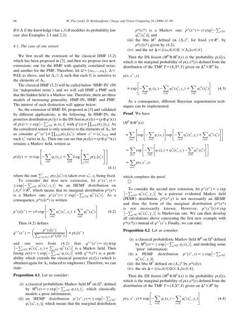
We first recall the extension <strong>of</strong> the classical HMF (3.2)<br />
which has been proposed in [3], <strong>and</strong> then we propose two new<br />
extensions: one for the HMF with spatially correlated noise,<br />
<strong>and</strong> another for the PMF. Therefore, let UZ{u 1 ,.,u k }, LZ<br />
P(U) as above, <strong>and</strong> let L 1 3L such that each Y s is sensitive to<br />
the elements <strong>of</strong> L 1 .<br />
The classical HMF (3.2) will be called below ‘HMF-IN’ (IN<br />
for ‘independent noise’), <strong>and</strong> we will call HMF a PMF such<br />
that the hidden field is a <strong>Markov</strong> one. Therefore, there are three<br />
models <strong>of</strong> increasing generality: HMF-IN, HMF, <strong>and</strong> PMF.<br />
The interest <strong>of</strong> such distinction will appear below.<br />
So, the extension <strong>of</strong> HMF-IN, proposed in [3] <strong>and</strong> validated<br />
by different applications, is the following. In HMF-IN, the<br />
posterior distribution p(xjy) is the DS fusion p(xjy)Z(p4q y )(x)<br />
<strong>of</strong> pðxÞZg exp K P <br />
c2C 4 c ðx c Þ with q y ðxÞf Q s2S pðy s jx s Þ.As<br />
the considered sensor is only sensitive to the elements <strong>of</strong> L 1 , let<br />
us consider q y; *ðx * Þf Q s2S pðy s jx s * Þ, where x * Zðx s * Þ s2S <strong>and</strong><br />
each x s * varies in L 1 . Then one can see that p(xjy)Z(p4q y *)(x)<br />
remains a <strong>Markov</strong> field, written as<br />
2<br />
2<br />
33<br />
pðxjyÞ Z g0 exp4K X 4 c ðx c Þ C X Log4<br />
X pðy s jx s * Þ55<br />
c2C<br />
s2S x s 2x s<br />
* (4.1)<br />
W. Pieczynski, D. Benboudjema / Image <strong>and</strong> Vision Computing 24 (2006) 61–69<br />
<br />
p*(x*) is a <strong>Markov</strong> one: p * ðx * ÞZg0 exp K P c2C<br />
4 0 * c ðx c * ÞŠ; <strong>and</strong><br />
(iii) the bba M 1 defined on (L 1 ) n , for fixed y2R n , by<br />
p*(yjx*) given by (4.2);<br />
(iv) <strong>and</strong> the set DZ{(u,A)2U !L 1 ju2A}.<br />
Then the DS fusion (M 0 4M 1 )(x) is the probability p(xjy),<br />
which is the marginal probability <strong>of</strong> p(x,x*jy) defined from the<br />
distribution <strong>of</strong> the TMF TZ(X,X*,Y) given on D n !R n by<br />
pðx; x * ; yÞ<br />
" #<br />
fexp K X c2C<br />
4 c ðx c ÞK X 4 c * ðx c * ; y c Þ C X 4 0 * c ðx c * Þ<br />
c2C<br />
c2C<br />
(4.3)<br />
As a consequence, different Bayesian segmentation techniques<br />
can be implemented.<br />
Pro<strong>of</strong>. We have<br />
ðM 0 4M 1 ÞðxÞ<br />
f X " "<br />
exp K X # "<br />
4 c ðx c Þ exp K X 4 c * ðx c * ;y c ÞC X ##<br />
4c 0* ðx c * Þ<br />
x2x * c2C c2C<br />
c2C<br />
" " ##<br />
Z X x2x * exp K X c2C<br />
Z X x2x * pðx;x * ;yÞ<br />
4 c ðx c ÞC4 * c ðx * c ;y c ÞK X c2C<br />
4 0*<br />
c ðx * c Þ<br />
where the sum P x s 2x s<br />
* pðy sjx s * Þ is taken over x s * , x s being fixed.<br />
To consider the first new extension, let p * ðx * ; yÞZ<br />
g exp K P <br />
c2C 4 c * ðx c * ; y c Þ be an HEMF distribution on<br />
(L 1 ) n !R n , which means that its marginal distribution p*(x*)<br />
is a <strong>Markov</strong> one: p * ðx * ÞZg 0 exp K P c2C 4 0 <br />
* c ðx c * Þ . As a<br />
consequence, p*(yjx*) is written<br />
"<br />
p * ðyjx * Þ Z g00 exp K X 4 c * ðx c * ; y c Þ C X #<br />
4 0 * c ðx c * Þ (4.2)<br />
c2C<br />
c2C<br />
Then (4.2) defines<br />
<br />
q y; *<br />
ðx * p<br />
Þ Z<br />
* ðyjx * Þ<br />
P<br />
x * 2ðL 1 Þ n p* ðyjx * Þ<br />
<br />
fpðyjx * Þ<br />
<strong>and</strong> one sees from (4.2) that q y; *ðx * ÞZgðyÞexp<br />
K P c2C 4 c * ðx c * ; y c ÞC P c2C 4 0 <br />
*<br />
<br />
c ðx c * Þ is a <strong>Markov</strong> field. Then<br />
fusing pðxÞZg exp K P <br />
c2C 4 c ðx c Þ with q y, *(x*) is a probability<br />
which extends the classical posterior p(xjy) (which is<br />
obtained again for L 1 reduced to singletons). Therefore, we can<br />
state:<br />
Proposition 4.1. Let us consider:<br />
(i) a classical probabilistic <strong>Markov</strong> field M 0 on U n , defined<br />
by M 0 ðxÞZg exp K P <br />
c2C 4 c ðx c Þ , which classically<br />
models a prior information;<br />
<br />
(ii) an HEMF distribution p * ðx * ; yÞZg exp K P c2C<br />
4 c * ðx c * ; y c ÞŠ, which means that the marginal distribution<br />
which completes the pro<strong>of</strong>.<br />
,<br />
To consider the second new extension, let p * ðx * ÞZg exp<br />
K P <br />
c2C 4 c * ðx c * ; y c Þ be a pairwise evidential <strong>Markov</strong> field<br />
(PEMF) distribution. p*(x*,y) is not necessarily an HEMF<br />
<strong>and</strong> thus the form <strong>of</strong> the marginal distribution p*(x*)<br />
is not necessarily known. However, p * ðx * jyÞfexp<br />
K P <br />
c2C 4 c * ðx c * ; y c Þ is <strong>Markov</strong>ian one. We can then develop<br />
all calculations above concerning the first new example with<br />
p*(x*jy) instead <strong>of</strong> q y,* (x * ). Finally, we can state:<br />
Proposition 4.2. Let us consider:<br />
(i) a classical probabilistic <strong>Markov</strong> field M 0 on U n defined<br />
by M 0 ðxÞZg exp K P <br />
c2C 4 c ðx c Þ , <strong>and</strong> modeling some<br />
‘prior’ information;<br />
<br />
(ii) a PEMF distribution p * ðx * ; yÞZg exp K P c2C<br />
4 c * ðx c * ; y c ÞŠ;<br />
(iii) the bba M 1 defined on (L 1 ) n by p*(xjy);<br />
(iv) the set DZ{(u,A)2U!L 1 ju2A}.<br />
Then the DS fusion (M 0 4M 1 )(x) is the probability p(xjy),<br />
which is the marginal probability <strong>of</strong> p(x,x*jy) defined from the<br />
distribution <strong>of</strong> the TMF TZ(X,X*,Y) given on D n !R n by<br />
"<br />
pðx; x * ; yÞfexp K X 4 c ðx c ÞK X #<br />
4 c * ðx c * ; y c Þ (4.4)<br />
c2C<br />
c2C


