Pairwise Markov Random Fields and its Application in Textured ...

Pairwise Markov Random Fields and its Application in Textured ImagesSegmentationWojciech Pieczynski and Abdel-Nasser TebbacheDépartement Signal et ImageInstitut National des Télécommunications,9, rue Charles Fourier, 91000 Evry, FranceE-mail Wojciech.Pieczynski@int-evry.frAbstractThe use of random fields, which allows one to take intoaccount the spatial interaction among random variables incomplex systems, is a frequent tool in numerous problemsof statistical image processing, like segmentation or edgedetection.In statistical image segmentation, the model is generallydefined by the probability distribution of the class field,which is assumed to be a Markov field, and the probabilitydistributions of the observations field conditional to theclass field. In such models the segmentation of texturedimages is difficult to perform and one has to resort to somemodel approximations. The originality of our contributionis to consider the markovianity of the pair (class field,observations field). We obtain a different model; inparticular, the class field is not necessarily a Markov field.The model proposed makes possible the use of Bayesianmethods like MPM or MAP to segment textured imageswith no model approximations. In addition, the texturedimages can be corrupted with correlated noise. Some firstsimulations to validate the model proposed are alsopresented.1. IntroductionWe propose in this paper a new Pairwise Markov RandomField model (PMRF), which is original with respect to theclassical Hidden Markov Random Field model (HMRF)[ChJ93]. The main difference is that in a PMRF the classfield is not necessarily a Markov field. One advantage,which will be developed in the following, is that texturedimages can be segmented without any modelapproximation.To be more precise, let S be the set of pixels, X = (X s) s∈Sthe random field of classes, and Y = (Y s) s∈Sthe randomfield of observations. The problem of segmentation is thenthe problem of estimating the realizations of the field Xfrom the observations of the realizations of the field Y .Prior to considering any statistical segmentation method,one must define the probability distribution P (X,Y)of therandom field (X,Y).In the classical HMRF model this distribution is given bythe distribution of X , which is a Markov field, and the setX=xP Yof the distributions of Y conditional to X = x .Under some assumptions on P X=x Y, the posteriorY=ydistribution P Xof X is a Markov distribution anddifferent Bayesian segmentation techniques like MPM[MMP87], MAP [GeG84] , or ICM [Bes86] can beapplied. These assumptions can turn out to be difficult tojustify when dealing with textured images, as detailed in[DeE87], [KDH88], [WoD92].The idea of the PMRF model we propose is to considerdirectly the Markovianity of the pairwise random fieldZ = (X,Y). The distribution of X is then the marginaldistribution of P (X,Y)and thus it is not necessarily aMarkovian distribution. What counts is that P Y=yXremainsMarkovian and so different Bayesian segmentationsspecified above can be used. When the particular problemof segmenting textured images with correlated noise isconsidered, the PMRF model is quite suitable becausedifferent Bayesian segmentation methods above can beapplied without any model approximation.The organization of the paper is following. In the nextsection we specify the difference between HMRF andPMRF in the case of simple Gaussian noise fields. Section3 is devoted to some simulations and some concludingremarks are presented in section 4.2. Pairwise Markov Random Field andtextured image segmentation2.1 Simple case of Hidden Markov FieldLet us consider the set of pixels S and X = (X s) s∈Sarandom field, each random variable X staking its values inthe class set Ω={ω 1,ω 2}. The field X is Markovian withrespect to four nearest neighbors if its distribution iswritten

⎡⎤P[X = x] = λ exp⎢− ∑ ϕ 1(x s, x t) − ∑ ϕ 2(x s) ⎥⎣⎢(s,t)neighborss ⎦⎥(2.1)where " (s,t) neighbors" means that the pixels s and t areneighbors and lie either on a common row or on a commoncolumn. The random field Y = (Y s) s∈Sis the field ofobservations and we assume that each Y stakes its values inR. The distribution of (X,Y) is then defined by (2.1) andthe distributions of Y conditional on X = x . Assumingthat the random variables (Y s) are independent conditionallto X and that the distribution of each Y sconditional toX = x is equal to its distribution conditional to X s= x s,we have :P[Y = yX= x] = ∏ f xs(y s)(2.2)swhere f xsis the density of the distribution of Y sconditional to X s= x s. Thus :P[X = x,Y = y] == λ exp[− ∑ ϕ 1(x s, x t) − ∑ [ϕ 2(x s) + Logf xs(y s)]] (2.3)(s,t)neighborssSo the pairwise field (X,Y) distribution is Markovian andthe distribution of X conditional to Y = y is stillMarkovian. It is then possible to simulate realizations ofX according to its distribution conditional to Y = y ,which affords the use of Bayesian segmentation techniqueslike MPM or MAP.In practice, the random variables (Y s) are not, in general,independent conditionally on X . In particular, (2.2) is toosimple to allow one to take texture into account. Forinstance, if we consider that texture is a Gaussian Markovrandom field realization [CrJ83], (2.2) should be replacedwith :P[Y = yX= x] == λ (x) exp[− ∑ a xs x ty sy t− 1(s,t)neighbors 22∑ [a xs x sy s+ b xsy s]] (2.4)The field Y is then Markovian conditionally on X , whichmodels textures. The drawback is that the product of (2.1)with (2.4) is not, in general, a Markov distribution. In fact,for the covariance matrix Γ(x) of the Gaussian distributionof Y = (Y s) s∈S(conditional to X = x ), we have :sMarkovianity invalidates the rigorous application of MPMor MAP.2.2 Simple case of Pairwise Markov FieldTo circumvent the difficulties above we propose to considerthe Markovianity of (X,Y). Specifically, we putP[X = x,Y = y] == λ exp[− ∑ ϕ[(x s, y s),(x t, y t)] − ∑ ϕ *[(x s, y s)]] =(s,t)neighborss= λ exp[− ∑ [ϕ 1(x s, x t) + a xs x ty sy t+ b xs x ty s+(2.6)(s,t)neighbors2+c xs x ty t] − ∑ [ϕ 2(x s) + a xs x sy s+ b xsy s]]sThe Markovianity of the pairwise field (X,Y) implies theMarkovianity of Y conditionally on X , and theMarkovianity of X conditionally on Y . The first propertyallows one to model textures, as in (2.4), and the secondone makes possible to simulate X according to itsposterior distribution, which allows us to use Bayesiansegmentation methods like MPM or MAP.Let us briefly specify how to simulate realizations of thepair (X,Y). The pair (X,Y) being Markovian, we canspecify the distribution of each (X s,Y s) conditionally onits neighbors. Let us consider the calculus of thedistribution of (X s,Y s) conditional to the four nearestneighbors :[(X t1,Y t1),(X t2,Y t2),(X t3,Y t3),(X t4,Y t4)] =[(x t1, y t1),(x t2, y t2),(x t3, y t3),(x t4, y t4)]This distribution can be written as(2.7)h(x s, y s) = p(x s) f xs(y s) (2.8)where p is a probability on the set of classes and, for eachclass x s, f xsis the density of the distribution of Y sconditional to X s= x s( p and f xsalso depend on(x t1, y t1),(x t2, y t2),(x t3, y t3),(x t4, y t4), which are fixed in thefollowing and so will be omitted). (2.8) makes thesampling of (X s,Y s) quite easy: one samples x saccordingto p, and then y saccording to f xs. We thus have:P{( X s,Y s) = (x s, y s)λ (x) = [(2π) N det(Γ(x))] −1/2 (2.5)which is not, in general, a Markov distribution withrespect to x .Finally, X is Markovian, Y is Markovian conditionallyon X , but neither (X,Y), nor X conditionally on Y , areMarkovian in general. This lack of the posterior[(X t1,Y t1),...,(X t4,Y t4)] = [(x t1, y t1),...,(x t4, y t4)]}∝ exp[− ∑ ϕ[(x s, y s),(x ti, y ti)] − ϕ *[(x s, y s)] =i=1,..., 4= exp[− ∑ [ϕ 1(x s, x ti) + a xs x tiy sy ti+ b xs x tiy s+i=1,..., 4+c xs x tiy ti] − [ϕ 2(x s) + a xs x sy 2 s+ b xsy s]](2.9)

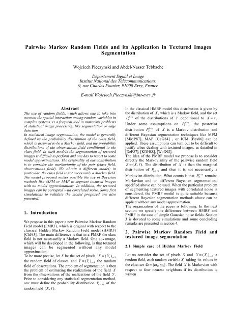
This can be written h(x s, y s) = p(x s) f xs(y s), where f xsisa Gaussian density defined by the following mean M xsand2variance σ xs:M xs=−∑b xs+ (a xs x tiy ti+ b xs x ti)i=1,..., 42a xs x s, σ xs2 =12a xs x s(2.10)and p the probability given on the set of classes with :p(x s) ∝(a xs x s) −1 exp[(b xs+ ∑ a xs x tiy ti+ b xs x ti) 2i=1,..., 44a xs x s−ϕ 2(x s) − ∑ (ϕ 1(x s, x ti) + c xs x tiy ti)]i=1,..., 4−(2.11)Finally, the main differences between the classical HMRFmodel and the new PMRF we propose are :(i) The distribution of X (its prior distribution) isMarkovian in HMRF and is not necessarily Markovian inPMRF;(ii) The posterior distribution of X is not necessarilyMarkovian in HMRF and is Markovian in PMRF;(iii) In the case of case of images which are textured, andpossibly corrupted with correlated noise, the PMRF allowsone to apply the Bayesian MPM or MAP methods withoutany model approximations.Remarks1. The classical HMRF can also be applied in the case ofmultisensor images [YaG95]. For m sensors theobservations on each pixel s ∈S are then assumed to be arealization of a random vector Y s= Y 1 m[ s,...,Y s ]. It ispossible to consider a multisensor PRMF. For example, amultisensor PMRF would be obtained by replacing in (2.6)2y sy tand y sby φ 1 [(y 1 s,...,y m s),(y 1 t,...,y m t)] andφ 2 [(y 1 s,...,y m s)].2. In some particular cases the classical model allows oneto take correlated noise into account [Guy93], [Lee98]. Thedifficulties arise when wishing to consider the cases whencorrelations vary with classes.2.3 General case of PMRFGeneralizing of the distribution given by (2.6) does notpose any problem. Let us consider k classesΩ={ω 1,...,ω k}, m sensors (each Y s= (Y 1 s,...,Y m s) takesits values in R m ), and C a set of cliques defined by someneighborhood system. The random field Z = (Z s) s∈S, withZ s= (X s,Y s), is a Pairwise Markov Random Field if itsdistribution may be written asP[Z = z] = λ exp[− ∑ ϕ c (z c)] (2.12)c∈CLet us note that the existence of the distribution (2.12) isnot ensured in a general case.In particular, three sensor PMRF can be used to segmentcolour images.RemarkAs mentioned above, X is not necessarily Markovian in aPMRF. This could be felt as a drawback, because thedistribution of X models the "prior" , i.e., without anyobservation, knowledge we have about the class image. Ofcourse, this "prior" distribution of X also exists in PMRF(it is the marginal distribution of P (X,Y)), but it is notMarkovian. The gravity of this "drawback" is undoubtedlydifficult to discuss in the general case. However, supposingthat it really is a drawback, let us mention that it alsoexists in the classical HMRF model. In fact, even in thevery simple case defined by (2.3), the observation field Yis not a Markov field. So, one could consider that the nonMarkovianity of X in the PMRF model is not strangerthat the non Markovianity of Y in the classical HMRFmodel.3. Visual examplesWe present in this section two simulations and twosegmentations by the MPM. We consider rather noisycases : one can hardly distinguish the class image in thenoisy one. One can notice that although the class imagesare not Markov fields realizations, they look like.The two realizations of PMRF presented in Fig.1 areMarkovian with respect to four nearest neighbors; thedistribution of (X,Y) is written :P[X = x,Y = y] == λ exp[− ∑ ϕ[(x s, y s),(x t, y t)] − ∑ ϕ *[(x s, y s)]] (3.1)(s,t)neighborsswithϕ[(x s, y s),(x t, y t)] = 1 2 (a x s x ty sy t+ b xs x ty s+ c xs x ty t+ d xs x t)(3.2)ϕ *[(x s, y s)] = 1 2 (α x sy 2 s+ β xsy s+ γ xs x t)The different coefficients in (3.2) are given in Tab.1. Let usnotice that it is interesting, in order to have an idea aboutthe noise level, to dispose of some information about thedistributions of Y conditional to X = x . In fact, these are

Gaussian distributions and knowing some parameters likemeans and variances can provide some information aboutthe noise level. Of course, the noise level also depends ondifferent correlations and the prior distribution of X .We may note that some of the coefficients in (3.2) aresimply linked with means or variances of the distributionsof Y conditional to X = x . In fact, denoting by Σ xthecovariance matrix of the Gaussian distribution of Yconditional to X = x and putting Q x= [q x st] s,t∈S=Σ −1 x, wehave :⎡P[Y = yX= x] ∝ exp − (y − m x )t Q x(y − m x) ⎤⎢⎣ 2⎥ (3.3)⎦Developing (3.3) and identifying to (3.2) we obtainImage 3 Image 6Fig. 1. Two realizations of Pairwise Markov Fields (Image1, Image 2), (Image 4, Image 5), and the MPMsegmentations of Image 2 (giving Image 3), and Image 5(giving Image 6), respectively.m xs=− β x s, σ 2 xs= 1(3.4)2α xsα xsImages 1, 2, 3 Images 4, 5, 6α xs1 1So, all other parameters being fixed, one can use (3.4) tovary the noise level. For instance, keeping the samevariances the noise level increases when one makes themeans approach each other. Otherwise, there are no simplelinks between correlations of the random variables (Y s)(conditionally on X = x ) and the coefficients in (3.2). Thecorrelations in Table 1, whose variations make appeardifferent textures, are estimated ones. The values of themeans show that the level of the noise is rather strong,which is confirmed visually.Image 1 Image 4Image 2 Image 5β xs−2m xs−2m xsγ xs x t2m xs2m xsa xs x t−0, 4 −0,1b xs x t−0, 4m xt−0,1m xtc xs x t−0, 4m xs−0,1m xsd xs x t0, 4m xsm xt+ ϕ(x s, x t) −0,1m xsm xt+ ϕ(x s, x t)m 1−0,3 1m 20,3 1,52σ 11 12σ 21 1ρ 110,26 0,05ρ 220,26 0,07τ 13,1% 07,9%Nb 30 × 30 30 × 30Tab.1α xs, ... , d xs x t: functions in (3.2), the function ϕ beingdefined by ϕ(x s, x t) =−1 if x s= x tand ϕ(x s, x t) = 1 ifx s≠ x t. m 1, m 2, σ 2 1, σ 2 2: the means and the variances in(3.3). ρ 11, ρ 22: the estimated covariances inter-class(neighboring pixels). τ : the error rate of wronglyclassified pixels with MPM. Nb = n 1n 2: the number ofiterations in MPM (the posterior marginals estimated fromn 1realizations, each realization obtained after n 2iterationsof the Gibbs Sampler).4 ConclusionsWe proposed in this paper an novel model called PairwiseMarkov Random Field (PMRF). A random field of classesX and a random field of observations Y form a PMRFwhen the pairwise random field Z = (X,Y) is a Markov