Estimation Of Generalized Mixtures And Its Application ... - IEEE Xplore

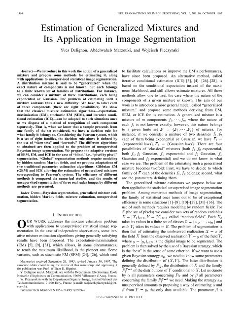
1364 IEEE TRANSACTIONS ON IMAGE PROCESSING, VOL. 6, NO. 10, OCTOBER 1997Estimation of Generalized Mixtures andIts Application in Image SegmentationYves Delignon, Abdelwaheb Marzouki, and Wojciech PieczynskiAbstract—We introduce in this work the notion of a generalizedmixture and propose some methods for estimating it, alongwith applications to unsupervised statistical image segmentation.A distribution mixture is said to be “generalized” when theexact nature of components is not known, but each belongsto a finite known set of families of distributions. For instance,we can consider a mixture of three distributions, each beingexponential or Gaussian. The problem of estimating such amixture contains thus a new difficulty: We have to label eachof three components (there are eight possibilities). We showthat the classical mixture estimation algorithms—expectationmaximization(EM), stochastic EM (SEM), and iterative conditionalestimation (ICE)—can be adapted to such situations onceas we dispose of a method of recognition of each componentseparately. That is, when we know that a sample proceeds fromone family of the set considered, we have a decision rule forwhat family it belongs to. Considering the Pearson system, whichis a set of eight families, the decision rule above is defined bythe use of “skewness” and “kurtosis.” The different algorithmsso obtained are then applied to the problem of unsupervisedBayesian image segmentation. We propose the adaptive versionsof SEM, EM, and ICE in the case of “blind,” i.e., “pixel by pixel,”segmentation. “Global” segmentation methods require modelingby hidden random Markov fields, and we propose adaptations oftwo traditional parameter estimation algorithms: Gibbsian EM(GEM) and ICE allowing the estimation of generalized mixturescorresponding to Pearson’s system. The efficiency of differentmethods is compared via numerical studies, and the results ofunsupervised segmentation of three real radar images by differentmethods are presented.Index Terms—Bayesian segmentation, generalized mixture estimation,hidden Markov fields, mixture estimation, unsupervisedsegmentation.I. INTRODUCTIONOUR WORK addresses the mixture estimation problemwith applications to unsupervised statistical image segmentation.In the case of independent observations, some iterativemixture estimation algorithms giving generally satisfyingresults have been proposed. The expectation-maximization(EM) [5], [9], [31], which allows, in some circumstances,to reach the maximum likelihood, is the pioneer one. Somevariants, such as stochastic EM (SEM) [24], [26], which tendManuscript received September 26, 1995; revised January 30, 1997. Theassociate editor coordinating the reivew of this manuscript and approving itfor publication was Prof. William E. Higgins.Y. Delignon and A. Marzouki are with the Département Electronique, ÉcoleNouvelle d’Ingénieurs en Communication, 59650 Villeneuve d’Ascq, France.W. Pieczynski is with the Département Signal et Image, Institut National desTélécommunications, 91000 Evry, France (e-mail: wojciech.pieczynski@intevry.fr).Publisher Item Identifier S 1057-7149(97)07026-7.to facilitate calculations or improve the EM’s performances,have since been proposed. An alternative method, callediterative conditional estimation (ICE) [3], [4], [26]–[28], isbased on the conditional expectation instead of the maximumlikelihood, and still allows estimate mixtures. All thesemethods allow one to treat the case where the nature of thecomponents of a given mixture is known. The aim of ourwork is to introduce a more general model, called “generalizedmixture,” and propose some methods deriving from EM,SEM, or ICE for its estimation. A generalized mixture is amixture of components where the nature ofeach is not known exactly; however, this nature belongsto a given finite setof natures. Forinstance, if we consider a mixture of two densitieseach of them being exponential or Gaussian, we haveexponential laws Gaussian laws There are fourpossibilities of “classical” mixtures (both exponential,both Gaussian, exponential and Gaussian,Gaussian and exponential) and we do not know in whatcase we are. The problem of the estimating such a generalizedmixture becomes twofold: First, we have to decide to whichfamily of each of the densities belongs; second, whatare the parameters defining them.The generalized mixture estimators we propose below arethen applied to the statistical unsupervised image segmentationproblem. Among numerous methods of image segmentation,the family of statistical ones turns out to be of exceptionalefficiency in some situations [1]–[8], [10]–[29], [31]–[36]. Theuse of such methods requires modeling by random fields: For(the set of pixels) we consider two sets of random variablescalled “random fields”. Eachtakes its values in a finite set of classesandeach takes its values in The problem of segmentation isthen that of estimating the unobserved realization ofthe field from the observed realization of the fieldwhereis the digital image to be segmented. Theproblem is then solved by the use of a Bayesian strategy, whichis the “best” in the sense of some criterion. If we want to use agiven Bayesian strategy , we need to know some parametersdefining the distribution of The latter distribution isgenerally defined by the distribution of and the familyof the distributions of conditional to Let us denoteby all parameters concerning and by all parametersconcerning the family we need. Making the strategyunsupervised amounts to proposing a way of estimating andfrom the only data available. The parameter is1057–7149/97$10.00 © 1997 IEEE

DELIGNON et al.: ESTIMATION OF GENERALIZED MIXTURES 1365generally of the form where defines thedistribution of conditional to If these distributionsare Gaussian, which is the most frequently considered case,each is of the form with being the meanand being the variance. The previous parameter estimationproblem is then the Gaussian mixture estimation problem. Inreal situations, the nature of the grey-level distribution canvary in time. For instance, the nature of the radar grey-leveldistribution of the sea surface depends on its state [8], thelatter depending on the weather. Thus, if we want to segmenta radar image where sea is one of the classes and we wishto dispose of an algorithm insensitive to weather conditions,we must consider the problem of estimating a generalizedmixture.The organization of the paper is as follows. In the next section,we address the generalized mixture estimation problemwithout reference to the image segmentation problem. Such amixture is defined and a method of its estimation based on theSEM is proposed.Section III contains a description of Pearson’s system, whichis a set of eight families of distributions, and different methodsfor estimating generalized mixtures whose components belongto this set are proposed. In fact, it is shown that the classicalmethods EM, SEM, or ICE can be generalized resulting ingeneralized EM, SEM, ICE (denoted by GEM, GSEM, GICE,respectively).In Section IV, we address the problem of unsupervisedimage segmentation, treating “local” and “global” methods.In the first case, GEM, GSEM, and GICE can be applieddirectly and we show that the use of their adaptive versionsis of interest. The second case, where the segmentation isperformed by the maximum posterior mode (MPM) [21],requires modeling by hidden Markov random fields. Differentparameter estimation methods have been proposed; let usmention Gibbsian EM [5], the algorithms of Zhang et al. [37],[38], stochastic gradient [35], the algorithm of Lakshmanan etal. [20], the algorithm of Devijver [16], and ICE. We considertwo of them (Gibbsian EM and ICE) and show that they canbe generalized in order to deal with the generalized mixturesestimation problem we are interested in.Section V contains results of some simulations, and segmentationsof three real radar images are presented.Conclusions are in the sixth section.II. GENERALIZED MIXTURE ESTIMATIONThe “classical” mixture estimation problem can be treatedwith methods like EM, SEM, or ICE. In this section, we willlimit our presentation to GSEM. Furthermore, for the sakeof simplicity, we shall consider the case of two classes andtwo families of distributions; its generalization is immediateand does not pose any problem. Let us note that the resultsof this section can be applied to any problem outside imagesegmentation.A. Classical Mixture Estimation and the SEM AlgorithmLet us suppose that the random variableswithare independent and identically distributed (i.i.d.),each taking its values in and inThe distributions of conditioned on areGaussiansrespectively. So, giventhe parameter defining the distribution ofisSEM is an iterative procedure thatruns as follows.1) Initialization: let be an initialguess of2) Calculation offromand, as follows.a) Compute, for each the distribution ofconditioned on If we denote by thebased densities this distribution is givenby(1)(2)b) Sample, for each a realization inaccording to the distribution above andconsiderthe “artificial” sampleof so obtained.c) Consider the partition ofdefined byd) Calculatebyand (3)3) Stop when the sequence stabilizes.B. Generalized Mixture EstimationLet us considera set of two families ofdistributions, a real random variable whose distributionbelongs either to or to anda sample of realizations of Let us temporarily assume thatwe dispose of a decision rule, which allows us todecide from in what set between and the distributionof lies. Such a decision rule, still called “ recognition,”will be made more explicit in what follows.(4)(5)

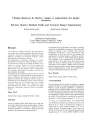
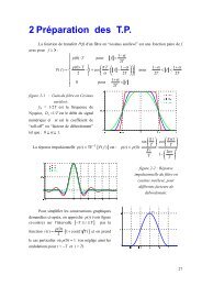
1366 IEEE TRANSACTIONS ON IMAGE PROCESSING, VOL. 6, NO. 10, OCTOBER 1997In order to simplify things, we expose the generalizedmixture estimation algorithm in the case of two classes andtwo possible families, but the generalization to any numberof classes and any number of possible families is quitestraightforward. Thus, we consider two random variableswhere takes its values in and in Thedistribution of is given byand the distributions of conditional to aregiven by densities , respectively. Let withthe Gaussian family and the exponential one. We assumethat is Gaussian or exponential andlikewise for Thus, we have four possibilities for “classical”mixture (both Gaussian, both exponential,Gaussian and exponential, exponential and Gaussian)and we do not know in what case we are. We observe a sampleof realizations of , and the problem is to1) estimate priors;2) choose between the four cases above;3) estimate the parameters of the densities chosen.The GSEM we propose runs as follows.1) Initialization.2) At each iterationa) sample as in the case of the SEM;b) apply, on and the rule determining thefamilies that and belong to;c) use and for estimating parameters (mean andvariance if the family is Gaussian, mean if the familyis exponential), in the same way that with SEM.Thus, the GSEM will be defined once we propose a decisionruleIn this paper, we will consider a well suited to thePearson family described in the next section; however, otherpossibilities exist [14].III. SYSTEM OF PEARSON ANDRECOGNITIONA. System of PearsonIn this section, we specify the family we will use in theunsupervised radar image segmentation and a decision ruleOur statement about Pearson’s system we will use is rathershort, and further details can be found in [17].A distribution density on belongs to Pearson’s systemif it satisfiesThe variation of the parametersprovides distributionsof different shape and, for each shape, defines theparameters fixing a given distribution. Let be a real randomvariable whose distribution belongs to Pearson’s system. Forlet us consider the moments of defined byand two parametersdefined by(6)(7)and (8)is called “skewness” and “kurtosis.”On the one hand, the coefficientsare related toby (10)–(13), shown at the bottom of the page.On the other hand, giventhe eight families of thesetwhose exact shape will be given in thenext section, are defined by(9)(14)The eight families are illustrated in the Pearson’s graphgiven in Fig. 1.What is important is that moments can be easilyestimated from empirical moments, from which we deducethe estimated values of by (9). Finally, we estimatethe family using (14). Once the family is estimated, valuesofgiven by (10)–(13) can be used to solvefor parameters defining the corresponding densities (given(10)(11)(12)(13)

DELIGNON et al.: ESTIMATION OF GENERALIZED MIXTURES 1367with(18)(19)Fig. 1.The eight families of Pearson’s system function of (1; 2):in Section III-B, where the shapes of the eight families arerecalled).Let us consider an i.i.d. sequence of real random variableswhose distribution belongs to Pearson’s system.We now specify the estimator used in step 2 of GSEM (seeSection II-B).1) Consider the partition of2) For each class use in order to estimate byParameters are called form parameters. cantake five different forms according to To be more precise1) for density is bell shaped;2) for density is shaped with;3) for density is shaped with;4) for density is shaped with;5) for density is uniform.(Type II Distributions): These distributions are particularcases of obtained for in (17), as follows:withforotherwise(20)(15)(21)(22)for (16)(Gamma Distributions):Densities are given by3) For each class calculate fromaccording to (9).4) For each class use and (14) to estimate whichfamily among the density belongs to.5) With the estimated family and the computed[(10)–(13)], estimate the parameters of the distribution.(For eachthe exact relationship betweendensity parameters and the computedisgiven in the next section.)with(Type IV Distributions):forDensities are given byotherwise(23)(24)B. Shape of Pearson’s System DensitiesIn this section, we specify the shape of the eight distributionfamilies forming Pearson’s system.(Beta Distributions of the First Kind): Densities aregiven byforotherwise(17)with such that and(25)

1368 IEEE TRANSACTIONS ON IMAGE PROCESSING, VOL. 6, NO. 10, OCTOBER 1997Fig. 2.Ring image, its noisy version, and results of unsupervised segmentations based on GGICE, GGEM, ASEM, and GSEM.(Inverse Gamma Distributions):Densities are given by(Gaussian Distributions): Densities are given bywithforotherwise(26)(Beta Distributions of the Second Kind): Densitiesgiven bywithforotherwiseare(27)withand(29)C. Generalized EM and ICE AlgorithmsThe EM and ICE algorithms are two other mixture estimationmethods that can also be “generalized” to give the GEMand GICE. We briefly describe below their operation.1) GEM: Let be the distributionscomputed fromthe current parameter Priors are reestimated by formula(30), which is the same as that in the EM algorithm, andthe recognition is the same as that the recognitiondescribed at the end of Section III-A, with the difference thatgiven forby formulas(31) and (32), are used instead of those given by formulas(15) and (16).(30)(31)where is the scale parameter and are the formparameters.(Type VII Distributions): Densities are given by(32)withsuch that(28)2) GICE: In the context of this paper, the GICE used isa “mixture” of GSEM and GEM. In fact, the reestimation ofpriors is the same as in GEM, and the family recognition andnoise parameter reestimation is the same as in GSEM.

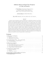
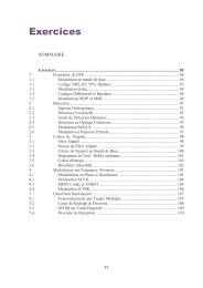
DELIGNON et al.: ESTIMATION OF GENERALIZED MIXTURES 1369B. Global Approach1) Markovian Model and Global Segmentation: In theglobal approach, each is estimated fromThe fieldis a Markov random field and we willconsider Ising’s model, which is the simplest one. In order tosimplify notations we will limit our presentation to the case oftwo classes; however, the generalization to any other numberof classes poses no particular problem.The distribution of is given bywithand(34)Fig. 3.Image 1: SEASAT image of the Brittany coast.if,if(35)IV. UNSUPERVISED IMAGE SEGMENTATIONIn this section, we propose some applications of differentgeneralized mixture estimators to the problem of unsupervisedimage segmentation. We shall consider two well known approaches:the “blind” approach and the “global” one. In theblind approach the generalized SEM, EM, and ICE algorithmsabove can be applied directly. In the global one we proposetwo adaptations of Gibbsian EM and ICE. For each methodwe specify here the reestimation formulas; the initialization ofdifferent algorithms is described in Section V.A. Blind ApproachThe “blind” approach consists of estimating the realizationof each from This is the simplest one and, generally,the least efficient. However, its “adaptive” version can be verycompetitive in some situations [26]. Let be priors andbe densities of the distribution of conditional toThe blind Bayesian strategy isifif(33)This strategy is made unsupervised by the direct use of theGSEM algorithm described above: One chooses a sequence ofpixels and considers that is the value of thegrey level at pixel In an “adaptive” version of the “blind”approach, one considers that priors depend on the positionof the pixel in The blind adaptive Bayesian strategy isthe same as above with instead of TheGSEM algorithm is modified as follows. Letbe the sequence obtained by sampling at a given iteration.In GSEM the priors are reestimated by the frequenciescomputed using all the sample points; in “adaptive” GSEM oneconsiders, for each a window centred at andare reestimated by frequencies computed from Letus note that in “adaptive” GSEM the sequence of pixelshas to cover In the following, the generalizedadaptive SEM, EM, and ICE will be denoted by GASEM,GAEM, and GAICE.Thus, is defined by The random variableswill be assumed independent conditionally to and furthermore,the distribution of each conditional to will beassumed equal to its distribution conditional on Underthese hypothesis all distributions of conditional to are definedby the two distributions of conditional torespectively. Let us denote by the densities of thesedistributions and assume that they belong to Pearson’s system.They are thus given by parametersand, respectively.Finally, all distributions of conditional to are definedby and thus defines the distributionofThe possibility of simulating realizations of according toits posterior, i.e. conditional to distribution constitutes themain interest of this model.2) Generalized Global ICE (GGICE): According to theICE principle, let us suppose that is observable. We havethen to proposeThere exist numerous estimators of the parameterfrom such as the coding method [2], the least squareserror method [12], or the maximum likelihood estimate [35].As our model is very simple, we can use an empiricalfrequency based estimator. In fact, there exists a simple linkbetween and probabilities “ knowing that theneighborhood of contains times,” where can take 0,1, 2, 3, 4 as values. For instance, if we take we select inthe image a sample of neighborhoods of containingtwo and two The probability “ knowing thatthe neighborhood of contains two ” is estimated by theproportion of the sample giving On the other handthis probability is given by(36)which gives an estimated value ofWe take for the same estimator as in the case ofindependent mixture, Section III-A.

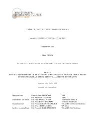
1370 IEEE TRANSACTIONS ON IMAGE PROCESSING, VOL. 6, NO. 10, OCTOBER 1997Fig. 4. Unsupervised segmentation results of Image 1, Fig. 3.Fig. 5.Image 2 and its unsupervised segmentations.Finally, the GGICE runs as follows.1) Sample according to .2) Compute .3) Consider andand apply 2–5 of the end of SectionIII-A.3) Generalized Gibbsian EM (GGEM)The difference between GGICE above and GGEM is situatedat the noise parameter reestimation level. We havetwo noise distributions conditional to the two classes and weare interested in estimating the four first moments of eachof them. In the case of GGICE, these two problems aretreated separately by considering the partition onandof the set ofpixels In the case of GGEM each of them is treated by theuse of the whole set Let us put(37)The first four moments of the noise corresponding to the firstclassare given byV. EXPERIMENTSWe present in this section some results of numerical applications.Let us note that in the global case the segmentation isperformed by the maximizer of posterior marginals (MPM)and, in the local case, it is performed by the rule (33).Thus, unsupervised segmentation algorithms considered in thispaper mainly differ by their parameter estimation step: Wewill note them by the parameter estimation method used. Forinstance, GEM will denote the local segmentation (33) basedon parameters estimated with generalized EM, GGEM willdenote the global MPM segmentation based on parametersestimated with generalized Gibbsian EM, and so on. The firstsection is devoted to synthetic images and in the second onewe deal with three real radar images.The initialization of GEM, GSEM, and GICE is as follows.We assume that we have a mixture of two Gaussian distributions.With denoting the cumulated histogram we takeandIn order to initialize GGEM and GGICE, we use thesegmentation obtained by the blind unsupervised method,which gives The noise parameters are initialized by thefinal parameters obtained in the parameter estimation step ofthe blind unsupervised method used.andforUse analogous formulas for the second class.(38)(39)A. Experiments on a Synthetic ImageLet us consider a binary image “ring” given in Fig. 2. Whiteis class 1 and black class 2. The class 1 is corrupted by a betanoise of the first kind (family in Pearson’s system) and theclass 2 is noised by a beta noise of the second kind (familyin Pearson’s system). The parameters defining the noisedistributions, their estimates with different methods, and thesegmentation error rates are given in Table I. The noisy versionof the ring image and some segmentation results are presentedin Fig. 2. We have taken the same means and variances on

DELIGNON et al.: ESTIMATION OF GENERALIZED MIXTURES 1371TABLE IPAR: PARAMETERS; TH:REAL VALUES OF PARAMETERS; ; 2 : MEAN AND VARIANCE; 1 ; 2 : SKEWNESS AND KURTOSIS;TYPE: FAMILY IN PEARSON’S SYSTEM; ERROR: SEGMENTATION ERROR RATE; ITE: NUMBER OF ITERATIONS OF ALGORITHMS. :PARAMETER OF THE MARKOV DISTRIBUTION OF X: GGICE: GLOBAL GENERALIZED ICE, GGEM: GENERALIZED GIBBSIAN EMTABLE IIPARAMETERS ESTIMATED FROM IMAGE 1, FIG. 3purpose: The human eye is essentially sensitive to the twofirst moments and, in fact, it is difficult to see anything in thenoisy version of the ring image.According to Table I, the behavior of the GSEM and theGICE is quite satisfactory when results obtained with GEMare clearly worse. In particular, GEM does not find the rightfamilies and Furthermore, the GSEM- and GICEbasedsegmentation error rates are very close to the theoreticalone. On the other hand, the behavior of both the GGICE andGGEM methods is very good. This is undoubtedly due toa good initialization with GSEM; however, the estimates ofskewness and kurtosis are still improved. We do not disposeof the theoretical segmentation error rate, as the ring image isnot a realization of a Markov field. However, the error ratesobtained seem quite satisfactory. As a conclusion, we may saythat the new difficulty of noise nature recognition is correctlytreated by the methods proposed, and the final segmentationquality is not affected significantly. We also present in Fig.2 the result of segmentation with generalized adaptive SEM(GASEM) whose quality is nearly comparable with the qualityof global methods. The result obtained with GSEM is verypoor compared to the results of global methods: This is notsurprising, and is due to the segmentation method and not tothe parameter estimation step.B. Segmentation of Real ImagesWe present in this section some examples of unsupervisedsegmentation of three real radar images. The first one, givenin Fig. 3, does not seem particularly noisy and adaptive localsegmentation seems to be competitive compared to globalmethods. The second one, given in Fig. 5, is more difficultto segment, and the third one, given in Fig. 7, is very noisy.From the results of Table II, we draw the following remarks.1) Starting from Gaussian distributions (type 8) GSEM,GEM and GICE all find beta distributions of the firstkind (kind 1) for both classes. Furthermore, all parametersget stabilised in these three methods at approximatelythe same values which can be relatively far fromthe initialized values. From this we may conjecture, onone hand, that real distributions are best represented bybeta distributions of the first kind and, on the other hand,that the parameters are correctly estimated.

1372 IEEE TRANSACTIONS ON IMAGE PROCESSING, VOL. 6, NO. 10, OCTOBER 1997Fig. 6. Segmentation of the Image 1 into four classes by generalized EM (GEM), generalized adaptive EM (GAEM), normal Gibbsian EM (NGEM),and generalized Gibbsian EM (GGEM).TABLE IIIPARAMETERS ESTIMATED FROM IMAGE 2, FIG. 52) Global methods keep beta distributions of the first kindgiven with the initialization by GSEM and thus we canimagine that these distributions are well suited to theimage considered.As in the case of the synthetic ring image, the GSEM-basedlocal segmentation, the only one represented on Fig. 4, givesvisually slightly better results that the GEM- and GICE-basedones. Parameters are perhaps better estimated but no clearexplanation appears when analyzing the results in Table II,apart from the fact that is close to values estimated byGGEM and GGICE. The use of adaptive GSEM improvesthe segmentation quality, which approaches the quality ofglobal segmentation methods. The efficiencies of the latterones appear quite satisfying (see Fig. 4).

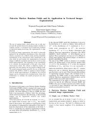
DELIGNON et al.: ESTIMATION OF GENERALIZED MIXTURES 1373Fig. 7. Image 3 (Amazonia) and its segmentation into three classes by generalized global ICE (GGICE), generalized adaptive ICE (GAICE), and classicaladaptive ICE, which uses Gaussian densities (NAICE).Concerning Image 2, all methods apart GSEM find betadistributions of the first kind (type 1) for the first classdistribution and beta of second kind (type 6) for the secondclass distribution; thus, we can reasonably assume that theyare well suited, among distributions of Pearson’s system, toreal distributions. Image 2 is rather noisy and the differencebetween global and local methods appears clearly. We notethat global methods provide visually better results that the localones, and, among the latter, the adaptive manner of parameterestimating provides some improvement.Let us briefly examine how the different methods work inthe case of more than two classes.We present in Fig. 6 the segmentations of the Image 1 intofour classes by GEM, GAEM, GGEM, and NGEM respectively.NGEM means “normal Gibbsian,” or “normal global”EM, in that no generalized mixture problem is considered andall noise densities are assumed Gaussian. Thus, note that GEMis generalized and local, and NGEM is traditional and global.According to Fig. 6, we note that GEM meanly indicates thepresence of two classes and, as in the case of two classessegmentation, the results obtained by GAEM are visually closeto the results, which means that the use of generalized mixtureestimation instead of the classical Gaussian mixture estimationcan have strong influence. Although their comparison isdifficult in the absence of the truth of the ground, we mayconjecture, as the Gaussian case is a particular case of thegeneralized one, that the results obtained with GGEM arebetter. As a curiosity, we note that the results obtained byGAEM look like the results obtained by NGEM.As a second example, we present in Fig. 7 some resultsof segmentation into three classes of an ERS 1 image of aforest area of Amazonia. ICE is the basic parameter estimationmethod used, and we compare GGICE, GAICE, and NAICE.As above, “N” means that only Gaussian densities are used,which means that NAICE is the traditional AICE. Image 3 isvery noisy and comparison between the results of the thesesegmentations is difficult in absence of the ground truth. Onlywe can say is that GGICE produces a result that seems visuallythe most consistent.VI. CONCLUSIONSWe have proposed in this work some new solutions to theproblem of generalized mixture estimation, with applicationsto unsupervised statistical image segmentation. A distributionmixture is said to be “generalized” when the exact nature ofcomponents is not known, but each of them belongs to a givenfinite set of families of distributions. The methods proposedallows one to1) identify the conditional distribution for each class;2) estimate the unknown parameters in this distribution;

1374 IEEE TRANSACTIONS ON IMAGE PROCESSING, VOL. 6, NO. 10, OCTOBER 19973) estimate priors;4) estimate the “true” class image.Assuming that each of unknown noise probability distributionis in the Pearson system, our methods are based onmerging two approaches of classical problems. On the onehand, we use classical mixture estimation methods like EM[5], [9], [31], SEM [24], [26], or ICE [3], [4], [26]–[28].On the other hand, we use the fact that if we know that thesample considered proceeds from one family in the Pearsonsystem, we dispose of decision rule, based on “skewness” and“kurtosis,” for which family it belongs to. Different algorithmsproposed are then applied to the problem of unsupervisedBayesian image segmentation in a “local” and “global” way.The results of numerical studies of a synthetic image andsome real ones, and other results presented in [22], show theinterest of the generalized mixture estimation in the unsupervisedimage segmentation context. In particular, the mixturecomponents are, in general, correctly estimated.As possibilities for future work, let us mention the possibilityof testing the methods proposed in many problems outsidethe image segmentation context, like handwriting recognition,speech recognition, or any other statistical problem requiringa mixture recognition. Furthermore, it would undoubtedlybe of purpose studying other generalized mixture estimationapproaches, based on different decision rules and allowing oneto leave the Pearson system.ACKNOWLEDGMENTThe image of Fig. 3 was provided by CIRAD SA underthe project GDR ISIS. The authors thank A. Bégué for hercollaboration.REFERENCES[1] R. Azencott, Ed., Simulated Annealing: Parallelization Techniques.New York: Wiley, 1992.[2] J. Besag, “On the statistical analysis of dirty pictures,” J. R. Stat. Soc.B, vol. 48, pp. 259–302, 1986.[3] B. Braathen, W. Pieczynski, and P. Masson, “Global and local methodsof unsuperivsed Bayesian segmentation of images,” Machine Graph.Vis., vol. 2, pp. 39–52, 1993.[4] H. Caillol, W. Pieczynski, and A. Hillon, “Estimation of fuzzy Gaussianmixture and unsupervised statistical image segmentation,” IEEE Trans.Image Processing, vol. 6, pp. 425–440, 1997.[5] B. Chalmond, “An iterative Gibbsian technique for reconstruction ofm-ary images,” Pattern Recognit., vol. 22, pp. 747–761, 1989.[6] R. Chellapa and R. L. Kashyap, “Digital image restoration using spatialinteraction model,” IEEE Trans. Acoust., Speech, Signal Processing, vol.ASSP-30, pp. 461–472, 1982.[7] R. Chellapa and A. Jain, Eds., Markov Random Fields. New York:Academic,1993.[8] Y. Delignon, “Etude statistique d’images radar de la surface de la mer,”Ph.D. dissertation, Université de Rennes I, Rennes, France, 1993.[9] A. P. Dempster, N. M. Laird, and D. B. Rubin, “Maximum likelihoodfrom incomplete data via the EM algorithm,” J. R. Stat. Soc. B, vol. 39,pp. 1–38, 1977.[10] H. Derin and H. Elliot, “Modeling and segmentation of noisy andtextured images using Gibbs random fields,” IEEE Trans. Pattern Anal.Machine Intell., vol. 9, pp. 39–55, 1987.[11] P. A. Devijver, “Hidden Markov mesh random field models in imageanalysis,” in Advances in Applied Statistics, Statistics and Images: 1.Abingdon, U.K.: Carfax, 1993, pp. 187–227.[12] R. C. Dubes and A. K. Jain, “Random field models in image analysis,”J. Appl. Stat., vol. 16, 1989.[13] S. Geman and G. Geman, “Stochastic relaxation, Gibbs distributions andthe Bayesian restoration of images,” IEEE Trans. Pattern Anal. MachineIntell, vol. PAMI-6, pp. 721–741, 1984.[14] N. Giordana and W. Pieczynski, “Estimation of generalized multisensorhidden Markov chains and unsupervised image segmentation,” IEEETrans. Pattern Anal. Machine Intell., vol. 19, pp. 465–475, 1997.[15] X. Guyon, “Champs aléatoires sur un réseau,” in Collection TechniquesStochastiques. Paris, France: Masson, 1993.[16] R. Haralick and J. Hyonam, “A context classifier,” IEEE Trans. Geosci.Remote Sensing, vol. GE-24, pp. 997–1007, 1986.[17] N. L. Johnson and S. Kotz, Distributions in Statistics: ContinuousUnivariate Distributions, vol. 1. New York: Wiley, 1970.[18] R. L. Kashyap and R. Chellapa, “Estimation and choice of neighborsin spatial-interaction models of images,” IEEE Trans. Inform. Theory,vol. 29, pp. 60–72, 1983.[19] P. A. Kelly, H. Derin, and K. D. Hartt, “Adaptive segmentation ofspeckled images using a hierarchical random field model,” IEEE Trans.Acoust., Speech, and Signal Processing, vol. 36, pp. 1628–1641, 1988.[20] S. Lakshmanan and H. Herin, “Simultaneous parameter estimationand segmentation of Gibbs random fields,” IEEE Trans. Pattern Anal.Machine Intell., vol. 11, pp. 799–813, 1989.[21] J. Marroquin, S. Mitter, and T. Poggio, “Probabilistic solution of illposedproblems in computational vision,” J. Amer. Stat. Assoc., vol. 82,pp. 76–89, 1987.[22] A. Marzouki, “Segmentation statistique d’images radar,” Ph.D. dissertation,Université de Lille I, Lille, France, Nov. 1996.[23] A. Marzouki, Y. Delignon, and W. Pieczynski, “Adaptive segmentationof SAR images,” in Proc. OCEAN ’94, Brest, France.[24] P. Masson and W. Pieczynski, “SEM algorithm and unsupervisedsegmentation of satellite images, IEEE Trans. Geosci. Remote Sensing,vol. 31, pp. 618–633, 1993.[25] E. Mohn, N. Hjort, and G. Storvic, “A simulation study of somecontextual clasification methods for remotely sensed data,” IEEE Trans.Geosci. Remote Sensing, vol. GE-25, pp. 796–804, 1987.[26] A. Peng and W. Pieczynski, “Adaptive mixture estimation and unsupervisedlocal Bayesian image segmentation,” Graph. Models ImageProcessing, vol. 57, pp. 389–399, 1995.[27] W. Pieczynski, “Mixture of distributions, Markov random fields andunsupervised Bayesian segmentation of images,” Tech. Rep. no. 122,L.S.T.A., Université Paris VI, Paris, France, 1990.[28] , “Statistical image segmentation,” Machine Graph. Vis., vol. 1,pp. 261–268, 1992.[29] W. Qian and D. M. Titterington, “On the use of Gibbs Markov chainmodels in the analysis of images based on second-order pairwiseinteractive distributions,” J. Appl. Stat., vol. 16, pp. 267–282, 1989.[30] H. C. Quelle, J.-M. Boucher, and W. Pieczynski, “Adaptive parameterestimation and unsupervised image segmentation,” Machine Graph. Vis.,vol. 5, pp. 613–631, 1996.[31] R. A. Redner and H. F. Walker, “Mixture densities, maximum likelihoodand the EM algorithm,” SIAM Rev., vol. 26, pp. 195–239, 1984.[32] A. Rosenfeld, Ed., Image Modeling. New York: Academic, 1981.[33] J. Tilton, S. Vardeman, and P. Swain, “Estimation of context for statisticalclassification of multispectral image data,” IEEE Trans. Geosci.Remote Sensing, vol. GE-20, pp. 445–452, 1982.[34] A. Veijanene, “A simulation-based estimator for hidden Markov randomfields,” IEEE Trans. Pattern Anal. Machine Intell., vol. 13, pp. 825–830,1991.[35] L. Younes, “Parametric inference for imperfectly observed Gibbsianfields,” Prob. Theory Related Fields, vol. 82, pp. 625–645, 1989.[36] J. Zerubia and R. Chellapa, “Mean field annealing using compoundGauss-Markov random fields for edge detection and image estimation,”IEEE Trans. Neural Networks, vol. 8, pp. 703–709, 1993.[37] J. Zhang, “The mean field theory in EM procedures for blind Markovrandom field image restoration,” IEEE Trans. Image Processing, vol. 2,pp. 27–40, 1993.[38] J. Zhang, J. W. Modestino, and D. A. Langan, “Maximum likelihoodparameter estimation for unsupervised stochastic model-based imagesegmentation,” IEEE Trans. Image Processing, vol. 3, pp. 404–420,1994.Yves Delignon received the Ph.D. degree in signalprocessing from the Université de Rennes 1, Rennes,France, in 1993.He is currently Associate Professor at the EcoleNouvelle d’Ingénieurs en Communication, Lille,France. His research interests include statisticalmodeling, unsupervised segmentation and patternrecognition in case of multisource data.

DELIGNON et al.: ESTIMATION OF GENERALIZED MIXTURES 1375Abdelwaheb Marzouki received the Ph.D. degreein signal processing from the Université des Scienceset Technologies de Lille, Lille, France, in1996. His Ph.D. was prepared at the École Nouvelled’Ingénieurs en Communication, Lille, and the InstitutNational des Télécommunications, Evry, France.He is mainly involved with unsupervised statisticalsegmentation of multisource images.Wojciech Pieczynski received the Doctorat d’Etatin mathematical statistics from the Université deParis VI, Paris, France, in 1986.He is currently Professor at the Institut Nationaldes Télécommunications, Evry, France. His researchinterest include mathematical statistics, statisticalimage processing, and theory of evidence.