Pairwise Markov Random Fields and its Application in Textured ...

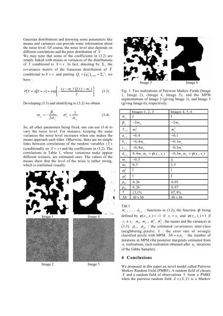
Gaussian distributions and knowing some parameters likemeans and variances can provide some information aboutthe noise level. Of course, the noise level also depends ondifferent correlations and the prior distribution of X .We may note that some of the coefficients in (3.2) aresimply linked with means or variances of the distributionsof Y conditional to X = x . In fact, denoting by Σ xthecovariance matrix of the Gaussian distribution of Yconditional to X = x and putting Q x= [q x st] s,t∈S=Σ −1 x, wehave :⎡P[Y = yX= x] ∝ exp − (y − m x )t Q x(y − m x) ⎤⎢⎣ 2⎥ (3.3)⎦Developing (3.3) and identifying to (3.2) we obtainImage 3 Image 6Fig. 1. Two realizations of Pairwise Markov Fields (Image1, Image 2), (Image 4, Image 5), and the MPMsegmentations of Image 2 (giving Image 3), and Image 5(giving Image 6), respectively.m xs=− β x s, σ 2 xs= 1(3.4)2α xsα xsImages 1, 2, 3 Images 4, 5, 6α xs1 1So, all other parameters being fixed, one can use (3.4) tovary the noise level. For instance, keeping the samevariances the noise level increases when one makes themeans approach each other. Otherwise, there are no simplelinks between correlations of the random variables (Y s)(conditionally on X = x ) and the coefficients in (3.2). Thecorrelations in Table 1, whose variations make appeardifferent textures, are estimated ones. The values of themeans show that the level of the noise is rather strong,which is confirmed visually.Image 1 Image 4Image 2 Image 5β xs−2m xs−2m xsγ xs x t2m xs2m xsa xs x t−0, 4 −0,1b xs x t−0, 4m xt−0,1m xtc xs x t−0, 4m xs−0,1m xsd xs x t0, 4m xsm xt+ ϕ(x s, x t) −0,1m xsm xt+ ϕ(x s, x t)m 1−0,3 1m 20,3 1,52σ 11 12σ 21 1ρ 110,26 0,05ρ 220,26 0,07τ 13,1% 07,9%Nb 30 × 30 30 × 30Tab.1α xs, ... , d xs x t: functions in (3.2), the function ϕ beingdefined by ϕ(x s, x t) =−1 if x s= x tand ϕ(x s, x t) = 1 ifx s≠ x t. m 1, m 2, σ 2 1, σ 2 2: the means and the variances in(3.3). ρ 11, ρ 22: the estimated covariances inter-class(neighboring pixels). τ : the error rate of wronglyclassified pixels with MPM. Nb = n 1n 2: the number ofiterations in MPM (the posterior marginals estimated fromn 1realizations, each realization obtained after n 2iterationsof the Gibbs Sampler).4 ConclusionsWe proposed in this paper an novel model called PairwiseMarkov Random Field (PMRF). A random field of classesX and a random field of observations Y form a PMRFwhen the pairwise random field Z = (X,Y) is a Markov