Pairwise Markov Random Fields and its Application in Textured ...

More documents

Recommendations

Info

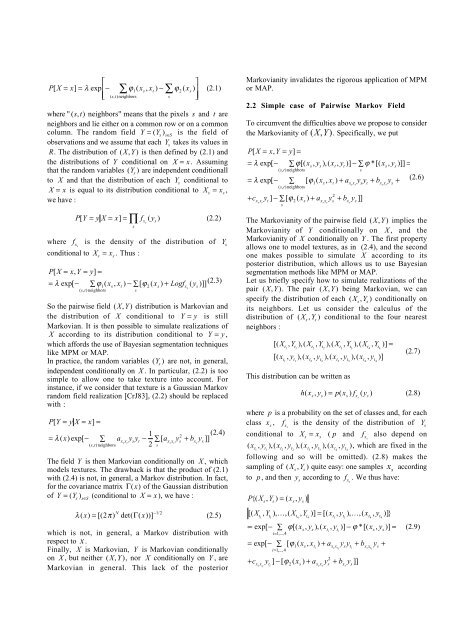
⎡⎤P[X = x] = λ exp⎢− ∑ ϕ 1(x s, x t) − ∑ ϕ 2(x s) ⎥⎣⎢(s,t)neighborss ⎦⎥(2.1)where " (s,t) neighbors" means that the pixels s and t areneighbors and lie either on a common row or on a commoncolumn. The random field Y = (Y s) s∈Sis the field ofobservations and we assume that each Y stakes its values inR. The distribution of (X,Y) is then defined by (2.1) andthe distributions of Y conditional on X = x . Assumingthat the random variables (Y s) are independent conditionallto X and that the distribution of each Y sconditional toX = x is equal to its distribution conditional to X s= x s,we have :P[Y = yX= x] = ∏ f xs(y s)(2.2)swhere f xsis the density of the distribution of Y sconditional to X s= x s. Thus :P[X = x,Y = y] == λ exp[− ∑ ϕ 1(x s, x t) − ∑ [ϕ 2(x s) + Logf xs(y s)]] (2.3)(s,t)neighborssSo the pairwise field (X,Y) distribution is Markovian andthe distribution of X conditional to Y = y is stillMarkovian. It is then possible to simulate realizations ofX according to its distribution conditional to Y = y ,which affords the use of Bayesian segmentation techniqueslike MPM or MAP.In practice, the random variables (Y s) are not, in general,independent conditionally on X . In particular, (2.2) is toosimple to allow one to take texture into account. Forinstance, if we consider that texture is a Gaussian Markovrandom field realization [CrJ83], (2.2) should be replacedwith :P[Y = yX= x] == λ (x) exp[− ∑ a xs x ty sy t− 1(s,t)neighbors 22∑ [a xs x sy s+ b xsy s]] (2.4)The field Y is then Markovian conditionally on X , whichmodels textures. The drawback is that the product of (2.1)with (2.4) is not, in general, a Markov distribution. In fact,for the covariance matrix Γ(x) of the Gaussian distributionof Y = (Y s) s∈S(conditional to X = x ), we have :sMarkovianity invalidates the rigorous application of MPMor MAP.2.2 Simple case of Pairwise Markov FieldTo circumvent the difficulties above we propose to considerthe Markovianity of (X,Y). Specifically, we putP[X = x,Y = y] == λ exp[− ∑ ϕ[(x s, y s),(x t, y t)] − ∑ ϕ *[(x s, y s)]] =(s,t)neighborss= λ exp[− ∑ [ϕ 1(x s, x t) + a xs x ty sy t+ b xs x ty s+(2.6)(s,t)neighbors2+c xs x ty t] − ∑ [ϕ 2(x s) + a xs x sy s+ b xsy s]]sThe Markovianity of the pairwise field (X,Y) implies theMarkovianity of Y conditionally on X , and theMarkovianity of X conditionally on Y . The first propertyallows one to model textures, as in (2.4), and the secondone makes possible to simulate X according to itsposterior distribution, which allows us to use Bayesiansegmentation methods like MPM or MAP.Let us briefly specify how to simulate realizations of thepair (X,Y). The pair (X,Y) being Markovian, we canspecify the distribution of each (X s,Y s) conditionally onits neighbors. Let us consider the calculus of thedistribution of (X s,Y s) conditional to the four nearestneighbors :[(X t1,Y t1),(X t2,Y t2),(X t3,Y t3),(X t4,Y t4)] =[(x t1, y t1),(x t2, y t2),(x t3, y t3),(x t4, y t4)]This distribution can be written as(2.7)h(x s, y s) = p(x s) f xs(y s) (2.8)where p is a probability on the set of classes and, for eachclass x s, f xsis the density of the distribution of Y sconditional to X s= x s( p and f xsalso depend on(x t1, y t1),(x t2, y t2),(x t3, y t3),(x t4, y t4), which are fixed in thefollowing and so will be omitted). (2.8) makes thesampling of (X s,Y s) quite easy: one samples x saccordingto p, and then y saccording to f xs. We thus have:P{( X s,Y s) = (x s, y s)λ (x) = [(2π) N det(Γ(x))] −1/2 (2.5)which is not, in general, a Markov distribution withrespect to x .Finally, X is Markovian, Y is Markovian conditionallyon X , but neither (X,Y), nor X conditionally on Y , areMarkovian in general. This lack of the posterior[(X t1,Y t1),...,(X t4,Y t4)] = [(x t1, y t1),...,(x t4, y t4)]}∝ exp[− ∑ ϕ[(x s, y s),(x ti, y ti)] − ϕ *[(x s, y s)] =i=1,..., 4= exp[− ∑ [ϕ 1(x s, x ti) + a xs x tiy sy ti+ b xs x tiy s+i=1,..., 4+c xs x tiy ti] − [ϕ 2(x s) + a xs x sy 2 s+ b xsy s]](2.9)
This can be written h(x s, y s) = p(x s) f xs(y s), where f xsisa Gaussian density defined by the following mean M xsand2variance σ xs:M xs=−∑b xs+ (a xs x tiy ti+ b xs x ti)i=1,..., 42a xs x s, σ xs2 =12a xs x s(2.10)and p the probability given on the set of classes with :p(x s) ∝(a xs x s) −1 exp[(b xs+ ∑ a xs x tiy ti+ b xs x ti) 2i=1,..., 44a xs x s−ϕ 2(x s) − ∑ (ϕ 1(x s, x ti) + c xs x tiy ti)]i=1,..., 4−(2.11)Finally, the main differences between the classical HMRFmodel and the new PMRF we propose are :(i) The distribution of X (its prior distribution) isMarkovian in HMRF and is not necessarily Markovian inPMRF;(ii) The posterior distribution of X is not necessarilyMarkovian in HMRF and is Markovian in PMRF;(iii) In the case of case of images which are textured, andpossibly corrupted with correlated noise, the PMRF allowsone to apply the Bayesian MPM or MAP methods withoutany model approximations.Remarks1. The classical HMRF can also be applied in the case ofmultisensor images [YaG95]. For m sensors theobservations on each pixel s ∈S are then assumed to be arealization of a random vector Y s= Y 1 m[ s,...,Y s ]. It ispossible to consider a multisensor PRMF. For example, amultisensor PMRF would be obtained by replacing in (2.6)2y sy tand y sby φ 1 [(y 1 s,...,y m s),(y 1 t,...,y m t)] andφ 2 [(y 1 s,...,y m s)].2. In some particular cases the classical model allows oneto take correlated noise into account [Guy93], [Lee98]. Thedifficulties arise when wishing to consider the cases whencorrelations vary with classes.2.3 General case of PMRFGeneralizing of the distribution given by (2.6) does notpose any problem. Let us consider k classesΩ={ω 1,...,ω k}, m sensors (each Y s= (Y 1 s,...,Y m s) takesits values in R m ), and C a set of cliques defined by someneighborhood system. The random field Z = (Z s) s∈S, withZ s= (X s,Y s), is a Pairwise Markov Random Field if itsdistribution may be written asP[Z = z] = λ exp[− ∑ ϕ c (z c)] (2.12)c∈CLet us note that the existence of the distribution (2.12) isnot ensured in a general case.In particular, three sensor PMRF can be used to segmentcolour images.RemarkAs mentioned above, X is not necessarily Markovian in aPMRF. This could be felt as a drawback, because thedistribution of X models the "prior" , i.e., without anyobservation, knowledge we have about the class image. Ofcourse, this "prior" distribution of X also exists in PMRF(it is the marginal distribution of P (X,Y)), but it is notMarkovian. The gravity of this "drawback" is undoubtedlydifficult to discuss in the general case. However, supposingthat it really is a drawback, let us mention that it alsoexists in the classical HMRF model. In fact, even in thevery simple case defined by (2.3), the observation field Yis not a Markov field. So, one could consider that the nonMarkovianity of X in the PMRF model is not strangerthat the non Markovianity of Y in the classical HMRFmodel.3. Visual examplesWe present in this section two simulations and twosegmentations by the MPM. We consider rather noisycases : one can hardly distinguish the class image in thenoisy one. One can notice that although the class imagesare not Markov fields realizations, they look like.The two realizations of PMRF presented in Fig.1 areMarkovian with respect to four nearest neighbors; thedistribution of (X,Y) is written :P[X = x,Y = y] == λ exp[− ∑ ϕ[(x s, y s),(x t, y t)] − ∑ ϕ *[(x s, y s)]] (3.1)(s,t)neighborsswithϕ[(x s, y s),(x t, y t)] = 1 2 (a x s x ty sy t+ b xs x ty s+ c xs x ty t+ d xs x t)(3.2)ϕ *[(x s, y s)] = 1 2 (α x sy 2 s+ β xsy s+ γ xs x t)The different coefficients in (3.2) are given in Tab.1. Let usnotice that it is interesting, in order to have an idea aboutthe noise level, to dispose of some information about thedistributions of Y conditional to X = x . In fact, these are
Page 1: Pairwise Markov Random Fields and i

Pairwise Markov Random Fields and its Application in Textured ...

You also want an ePaper? Increase the reach of your titles

Delete template?

Save as template?