Numerical simulation of sediment mixture deposition part 1 ... - LTHE

More documents

Recommendations

Info

2 SEDICOUP modeling system SEDICOUP is a 1-D modeling system for river sedimentation engineering. General features of the software have not varied since its previous versions (Holly and Rahuel, 1990, Belleudy, 1992). Basically, SEDICOUP performs the solution of unsteady de Saint-Venant flow equations coupled with a generalized form of Exner equation for global bed-material conservation and transport equations of graded sediments. Sediment mixture is described through a breakdown into sediment size classes. Bed material sorting equations link exchanges between sediment transport, the active layer of the bed (the so-called mixing layer), and the underneath strata. Present characteristics of the software were developed for its application in engineering studies. In particular its modularity allows addition, or suppression, of equations, depending on their importance in the current application. For the calculations that are presented in the present paper, only bed-load transport is considered. Suspended load equations (as presented by Holly and Rahuel, 1990) are dropped off. For the formulation of physical processes, different sets of empirical formulations have been implemented in order to adapt the modeling to the characteristics of the application. Bed-load transport Selection among the different formulations available in SEDI- COUP for sediment load will be in Part 2. The simulation presented within this paper uses the formulation by Engelund and Hansen (1967) (EH) for bed-load (or total load in the case where suspended load is not considered). This formulation is well suited for the sediment and shear stress characteristics met in our case, although some discussion could be done in the case of flume scales. Our objective was not the calibration of this formulation for a perfect fitting with measurements but rather discussion about coupling effects between deposition rate and grain mixture. A good agreement of the simulation results with the measurements was nevertheless obtained, as can be seen in the following when using usual coefficients. SEDICOUP computes transport load separately for each of the sediment size classes. A classical adaptation of the usual EH formulation for mean diameter d m is done. The representative diameter d j of the sediment size class replaces diameter d m . Relative presence of class j within the bed surface layer is taken into account with factor β j which is net volumetric fraction of sediment j. Net volumetric sediment discharge g v,j of size class j, per unit width, is: g vj 0.1β j g ρ 5/ s – ρ 2 3θ = -------------d j ρ j -------- f EH 2S f f 2ghS EH = ------- = ------------- f Fr 2 V 2 (1) with g, the gravitational acceleration; ρ s , ρ the specific weight of sediment and water, respectively; d j the diameter of bed material ; f EH the friction factor ; S f the energy slope ; Fr the Froude number ; and h the water depth. The dimensionless shear stress θ j is itself a function of sediment diameter d j: hS θ j = ------------------ f (2) ρ s – ρ -------------d ρ j Implementation of an additional term for hiding/exposure effects will be discussed in Part 2. From equation (1), the total sediment transport rate capacity G j * (g v,j summed over "active width") is directly a function of flow characteristics, and of bed surface grain distribution β j . In SEDICOUP, G j * is the sediment transport rate that would be achieved if equilibrium was reached. Taking this value as the actual transport rate is not satisfactory (for example in the case of the present experiment) because, obviously, it does not reproduce upstream input of sediment and drag and deposition of this overload especially within the first meters of the flume. In the modeling, the actual sediment transport rate G j is linked to the potential transport rate G j * through the so-called loading law: ∂G -------- j PG ( ∂x j – G j ) ----- G j ∂G * – – -------- j = 0 (3) ∂x G j * The idea, and the formulation of the loading law equation (a sort of space lag equation), was introduced after Daubert and Lebreton (1967) and Bell and Sutherland (1983), the former limiting their formulation to the first two terms of (3). Loading law equations are introduced in the system of equations for each j of the J sediment size classes. In the present simulation, the complete formulation has been used, with a constant loading parameter P=1/∆x, identical for all sediment size classes. As the sensitivity analysis to this loading parameter is not performed later in this paper, and in order to appreciate the effect of the loading law, we display in Figure 11 potential transport rate and effective transport rate (total) at a given time of a simulation. Mixing layer and strata One single reference-layer is considered at the surface of the bed for computation of sediment fluxes. According to the definition provided in the literature, SEDICOUP is a single-layer model (Di Silvio 1991, Sieben 1996), or 3 or 4 layer model (according to the definition of Peviani 1992, who takes account of transport layers), depending on an option which is selected (bed-load only or bed-load and suspended load). The so-called "mixing" layer is, in SEDICOUP formulation, a characteristic control volume where volumetric fraction β j controls availability for transport of sediment of class j. This is 418 JOURNAL DE RECHERCHES HYDRAULIQUES, VOL. 38, 2000, NO. 6
done through the presence of β j in equation (1) for transport capacity g v,j *. The bed material sorting equation is: with p the porosity of bed material; w act the width of the "active bed"; e m the mixing layer thickness; G j the total net volumetric sediment discharge of class j; Γ the alluvial bed area with respect to a reference plane; S j a source term (exchanges with suspended load, bank aggradation/degradation, lateral input). 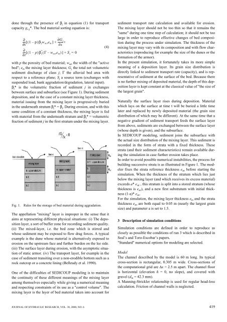β j * is the volumetric fraction of sediment j in exchanges between surface and subsurface (see Figure 1). During sediment deposition, and in the case of a constant mixing layer thickness, material issuing from the mixing layer is progressively buried in the underneath stratum β j * = β j . During erosion, and with this same condition of a constant thickness, the mixing layer is fed with material from the underneath stratum and β j * = volumetric fraction of sediment j in the first stratum under the mixing layer. Fig. 1. ∂ ∂G ---- [( 1– p) β ∂t j w act e m ] + --------+ j ∂x ∂ ---- [( 1 – p) β * ∂t j ( Γ – w act e m )] + S j = 0 Rules for the storage of bed material during aggradation. (4) The appellation "mixing" layer is improper in the sense that it aims at representing different physical situations: (i) The deposition layer, a sort of buffer zone for recording sediment quality. (ii) The mixed-layer, i.e. the bed zone which is stirred and whose sediment may be exposed to flow drag forces. A typical example is the dune whose material is alternatively exposed to erosion on the upstream face and further burden on the lee side. (iii) The surface layer during erosion, with the asymptotic situation of static armor. (iv) The transport layer, for example in the case of sediment transiting over a non-erodible bottom such as a rock outcrop or a concrete lining (Belleudy et al. 1990). One of the difficulties of SEDICOUP modeling is to maintain the continuity of these different meanings of the mixing layer among themselves especially while giving a numerical meaning and respecting constraints of its use as a "control volume". The mixing layer is the layer of bed material taken into account for sediment transport rate calculation and available for erosion. The mixing layer should not be too thin so that it remains the "same" during one time step of calculation; it should not be too large in order to reproduce effective changes of bed composition during the process under simulation. The thickness of the mixing layer may vary with its composition and with flow characteristics (reproducing for example the size of the dunes or the formation of the armor). In the present simulation, it fortunately takes its more simple meaning of a deposition layer. Its grain size distribution is directly linked to sediment transport rate (capacity), and is representative of sediment at the surface of the bed. Because there is no further mixing of deposited material, the depth of this deposition layer is kept constant at the classical value of "the size of the largest grain". Naturally the surface layer rises during deposition. Material which lays on the surface at time t will be buried a little time later and replaced by newly deposited material (the grain size distribution of which may be different). At the same time that a negative gradient of sediment transport feeds the surface layer from above, sediments are exchanged between the surface layer (whose depth is given), and the subsurface. In SEDICOUP modeling, sediment joins the subsurface with the actual size distribution of the mixing layer. This sediment is recorded in the form of strata with a fixed thickness. These strata (and their sediment characteristics) remain available during the simulation in case further erosion takes place. In order to avoid possible numerical instabilities, the process for building successive strata is as illustrated in Figure 1. The modeler fixes the strata reference thickness e str before starting the simulation. When the thickness of the stratum which lies just below the mixing layer (and which receives its excess material) exceeds a* e str , this stratum is split into a stored stratum (whose thickness is e str ), and a new first substratum with initial thickness (1-a)* e str . For the simulation, the mixing layer thickness e m and the strata thickness e str are both equal to 0.05 m (nearly the largest grain size) and parameter a is set to 1.5. 3 Description of simulation conditions Simulation conditions are defined in order to reproduce as closely as possible the conditions of run 3 which is described in Seal’s and Toro-Escobar’s papers. "Standard" numerical options for modeling are selected. Model The channel described by the model is 60 m long. Its typical cross-section is rectangular, 0.305 m wide. Cross-sections of the computational grid are ∆x = 2.5 m apart. The channel floor is horizontal (elevation h = 0, no slope), and covered with gravel (d m = 42.3 mm). A Manning-Strickler relationship is used for regular head-loss calculation. Friction of channel walls is neglected. JOURNAL OF HYDRAULIC RESEARCH, VOL. 38, 2000, NO. 6 419
Page 1: Numerical simulation of sediment mi
Page 5 and 6: Front elevation is very similar to
Page 7 and 8: the reference for bed load calculat
Page 9 and 10: Appendix 1: Characteristics the sim

Numerical simulation of sediment mixture deposition part 1 ... - LTHE

Create successful ePaper yourself

Delete template?

Save as template?