FEMLAB - KTH

Mathematical Modelling
and Numerical Solution of Chemical
Reactions and Diffusion of Carcinogenic
Compounds in Cells
DONALD O BESONG
Master’s Degree Project
Stockholm, Sweden 2004
TRITA-NA-E04152

Numerisk analys och datalogi Department of Numerical Analysis
KTH and Computer Science
100 44 Stockholm Royal Institute of Technology
SE-100 44 Stockholm, Sweden
Mathematical Modelling
and Numerical Solution of Chemical Reactions
and Diffusion of Carcinogenic Compounds in Cells
DONALD O BESONG
TRITA-NA-E04152
Master’s Thesis in Numerical Analysis (20 credits)
at the Scientific Computing International Master Program,
Royal Institute of Technology year 2004
Supervisor at Nada was Michael Hanke
Examiner was Axel Ruhe

Abstract
In order to shed more light on how cancer is triggered, Professor Bengt Jernstrom
and his research group at Karolinska Institute (KI) have been performing
in vitro incubation of carcinogenic compounds with cells. In vitro reactions and
diffusion take place when the carcinogenic substrate is added to cells in culture.
Only one cell and its appropriate quota of the medium is needed for the mathematical
model, and indeed only a 22.5 o sector of a cell is modelled. FEMLAB is
the software used for the simulation. The graphical representation of the problem
and its simulation is made possible by applying the mathematical technique of homogenisation
in the multi-compartment cytoplasm. All constants and parameters
used in the simulation were the same used for the in vitro experiments. The model,
and consequently the programme, can be adapted to various physical and chemical
scenarios.
The concentration of the carcinogenic substrate in the extracellular solution is
computed, and its half-life is compared to the in vitro results. Both results are found
to be the same.
The model can be used for the prediction of the experimental inaccessible concentration
profile in the nucleus.
Matematisk modellering och numerisk lösning av
reaktioner och diffusion för cancerogena ämnen i
celler
Sammanfattning
För att belysa hur cancer uppkommer, har prof Bengt Jernström och hans forskargrupp
p˚a Karolinska Institutet (KI) utfört in vitro odling av cancerogena ämnen
i celler, där reaktioner och diffusion d˚a äger rum. Endast en cell behövs för att
sätta upp en matematisk modell, och av denna cell modelleras endast en 22.5
graders sektor. FEMLAB har använts för simuleringen. Den grafiska representationen
av problemsimuleringen har möjliggjorts genom att applicera homogenisering

p˚a multi-compartment cytoplasma. Alla konstanter och parametrar som använts i
modellen hade samma värden som i in vitro experimenten. Modellen, och även programmet,
kan anpassas till olika fysikaliska och kemiska scenarier. Koncentrationen
av de cancerogena ämnena i modellen och deras halvtids livslängder beräknas
och jämförs med in vitro resultat. B˚ada resultaten överensstämmer. Modellen kan
användas för prediktion av omätbara koncentrationer i cellkärnan.

Contents
1 Introduction 1
2 The Physical Problem and its Mathematical Model 3
2.1 Diffusion . . . . . . . . . . . . . . . . . . . . . . . . . . . . . . 4
2.2 Reaction . . . . . . . . . . . . . . . . . . . . . . . . . . . . . . . 4
2.3 Initial Conditions . . . . . . . . . . . . . . . . . . . . . . . . . . 5
2.4 Boundary Conditions . . . . . . . . . . . . . . . . . . . . . . . . 5
3 Scaling and Reformulation 7
3.1 The diffusion reaction model equation . . . . . . . . . . . . . . . 8
4 Simplification of problem by means of homogenisation 9
4.1 Finding D eff . . . . . . . . . . . . . . . . . . . . . . . . . . . . 10
4.1.1 Weighted arithmetic mean of the diffusion coefficient . . . 10
4.1.2 Weighted harmonic mean diffusion coefficient . . . . . . 11
4.1.3 Decision on D eff for the cytoplasm . . . . . . . . . . . . 12
4.2 Partition coefficient between homogenised cytoplasm and other subdomains
. . . . . . . . . . . . . . . . . . . . . . . . . . . . . . . 12
4.3 Solving for concentration; Fraction of C undergoing chemical reaction
. . . . . . . . . . . . . . . . . . . . . . . . . . . . . . . . 13
4.3.1 Reaction. Fraction of concentration affected by chemical
reaction in the cytoplasm. . . . . . . . . . . . . . . . . . 13
5 Model Implementation with FEMLAB 15
5.1 The Femlab Software . . . . . . . . . . . . . . . . . . . . . . . . 15
5.2 The Geometry . . . . . . . . . . . . . . . . . . . . . . . . . . . . 15
5.3 Subdomain properties, equations and constants . . . . . . . . . . 16
5.4 Constants and Parameters . . . . . . . . . . . . . . . . . . . . . . 17
5.5 Subdomains and their properties . . . . . . . . . . . . . . . . . . 17
5.6 Initial condition . . . . . . . . . . . . . . . . . . . . . . . . . . . 19
5.7 Boundary conditions . . . . . . . . . . . . . . . . . . . . . . . . 19
5.8 Solving . . . . . . . . . . . . . . . . . . . . . . . . . . . . . . . 19

5.9 Results . . . . . . . . . . . . . . . . . . . . . . . . . . . . . . . 20
6 Conclusion 22
References 24
List of Abbreviations 25

Chapter 1
Introduction
The aim of this work is to develop a mathematical model for the in vitro chemical
reactions and diffusion of carcinogenic compounds in cells, and then create a computer
programme based on the model. Consequently, by using different parameters
the programme will enable us to carry out these experiments virtually, and thus
predict the risk of cancer in living humans and animals.
The primary carcinogenic substrate, in the form of diol epoxides (C), is initially
outside the cell. Outside the cell, some of this substrate reacts with water to form
tetrols (U), which do not cause cancer, although it diffuses everywhere in the cell.
When the remaining substrate C diffuses through the outer membrane of the cell,
it still reacts with water within the cytoplasm, while some of it is converted into
glutathione conjugates (B) by an enzyme called GST . B does not cause cancer
either, but remains in the cytoplasm, where it is pumped out. The remaining C will
reach the nucleus, where it still reacts with water in the nucleus to form U, as well
as with DNA to form DNA adducts (A). It is this A that causes cancer. It will stay
in the nucleus without diffusing into the other parts of the cell.
Each cell in the cell culture used in the study is surrounded by about 168 times
its volume of medium. The substrate was then added in the medium for the reactions
and diffusion to begin.
There are no reactions in the membranes, or so-called lipid compartment of
the cell. Reaction only takes place in the aqueous compartment of the cell: In the
cytoplasm the reaction of substrate C with water is slow but the enzymatic reaction
is much faster. In the nucleus, the reaction of C with DNA is the same rate as the
reaction with water in the cytoplasm.
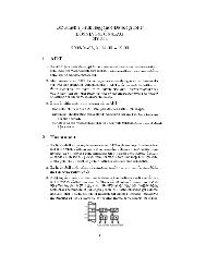
Figure 1.1 illustrates the diffusion and reactions in and out of a cell.
The partition coefficient, Kp, which is the equilibrium ratio of the concentration
C or U between any aqueous compartment of the cell and its neighbouring lipid
compartment, is 1 × 10 −3 . Kp depends on the substrate.
The complexity of this work lies on the complex geometry, as well as the fact
1

Figure 1.1. Illustration of reactions and diffusion in a cell
that there are many reactions with different products, and their diffusion, in each
part of the cell. With mass transfer between various parts of the cell, the work has
proved to be more complex, but the bottle-neck is a geometry with heavily varying
details. This is handled by applying scaling and homogenisation. We shall go into
this after studying the physical domain as presented in chapter 2, which reveals
the cytoplasm as consisting of thousands of interconnected tiny parts of the lipid
compartment sandwiched between very tiny parts of the aqueous compartment.
Chapter 2 sets the physical problem and formulates its mathematical model. It
is most important to work with a dimensionless model, so in Chapter 3, the model
is scaled and reformulated. In Chapter 4, the homogenisation of the cytoplasm is
explained, as well as how the solution of the modified problem is obtained with
a knowledge of equilibrium isotherms [7, pp.407,408]. A brief presentation of the
FEMLAB software is found in Chapter 5, where the implementation of the model is
described. Also in Chapter 5, there is a list of the variable names in the programme,
with their physical meanings, so that users of the programme may easily adapt it to
their own needs.
The in vitro experiments were performed by Kristian Dreij, who is presently a
PhD student of toxicology under the supervisors prof. Bengt Jernstrom and prof.
Ralf Morgenstern at K.I. They all, as well as my supervisor at KT H doc. Michael
Hanke, have always been quick to help me in this work.
2

Chapter 2
The Physical Problem and its
Mathematical Model
The concentration of the cells in the culture is one cell per 168 times its volume
of the medium. Therefore, the smallest useful part of the physical domain for this
study is a cell surrounded by about 168 times its volume of the substrate solution.
Originally, the substrate C is found only in this extra-cellular solution.
The cell consists of the cell membrane which has a thickness of 0.16 percent of
the radius of the nucleus. Beyond the cell membrane is the cytoplasm which has
a thickness of 3 times the radius of the nucleus, and the nuclear membrane which
has the same thickness as the cell membrane. At the centre of the cell we have the
nucleus, 4.8 × 10 −6 m in radius.
We shall call the outer and nuclear membranes, together with the inner membranes
within the cytoplasm, the lipid compartment of the cell, and the rest of the
cell the aqueous compartment, which comprises both the cytoplasm and nucleus
minus any membranes therein. Note that this aqueous compartment of the cell is
not the same as the extracellular water.
The cytoplasm contains thousands of inter-connected membrane-like sheets,
as well as tiny structures consisting of membranes of the same thickness as the
outer membrane. Examples of these structures are the endoplasmic reticulii and the
mitochondria. Some of these structures are closed and oval in shape, but contain
a aqueous compartment. The nucleus is free from any membranes. However, the
ratio of all the lipid compartment of the cell to the volume of the whole cell is
about 25 : 100. That is, one quarter of the cell is made up of these membranes.
Moreover, since the scaled radius of the whole cell is 4, the scaled thickness of the
cytoplasm 3, and the radius of the nucleus 1, and all these membranes are found in
the cytoplasm except the cell membrane and the nuclear membrane which can be
neglected, the volume fraction of the lipid compartment in the cytoplasm is given
3

y
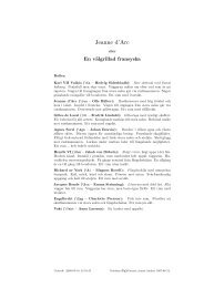
Figure 2.1. Schematic picture of the cell showing cytoplasm and nucleus
�
43 0.25
43 − 13 �
= 0.254 (2.1)
The cytoplasm is therefore packed with membranes, as can be seen in Figure
2.1.
This is a diffusion/reaction problem. There is no advection. I will first describe
the diffusion modelling and then the reaction modelling. Finally, I will combine
them.
2.1 Diffusion
Let us call the ith subdomain Ωi, and let us assume that the concentration of the
diffusing species in Ωi is φ. Let the diffusion coefficient of φ in Ωi be D. Then, the
rate of change of φ in Ωi is given by
2.2 Reaction
∂φ
∂t = D ▽2 φ (2.2)
In this study, C is the only compound which reacts. Let the concentration of C, B, U
and A in Ωi be denoted by Ci, BiUi and AiCi respectively. There are three reactions:
4

Ci + water −→ Ui at rate kiCi
(2.3)
where ki is the rate constant of the reaction with water in the ith subdomain subdomain.
Ci + GST −→ Bi at rate kBiCi · GST (2.4)
where the enzyme GST has so many active sites that the reaction rate is always
constant.
Ci + DNA −→ Ai at rate kAiCi (2.5)
kAi and kBi are the rate constants of the reaction with A and B respectively in the
ith subdomain subdomain. If a certain reaction does not take place in some subdomain
Ωi, then the appropriate reaction rate is simply 0. For example, there are no
reactions in the lipid compartment of the cell (membranes), so all the reaction rates
there are 0.
For instance, in the nucleus Ωnu, the models for the reactions represented by
(2.3) and (2.5) are:
dCnu
dt = −(knu + kAnu)Cnu (2.6)
where the subscript nu indicates that the variable belongs to the nucleus.
2.3 Initial Conditions
dUnu
dt = +knuCnu (2.7)
dAnu
dt = +kAnuCnu (2.8)
In all the subdomains, the initial concentration is 0 for all the substances C,U,B,
and A, except that the initial concentration of C in the rectangular domain Ω0 representing
the extracellular solution, is C0.
2.4 Boundary Conditions
On the left boundary of the rectangular subdomain we have a homogeneous boundary
condition because of symmetry. On its upper and lower boundaries we also
have homogeneous boundary condition because there are no concentration gradients
along their normals. The upper and lower boundaries of the sector-like geometry
to the right of the rectangular subdomain we also have zero Neumann boundary
5

conditions because there are no concentration gradients in the direction of their
normals. Hence, for any species φi at those boundaries, the flux is given by:
n · (D ▽ φi) = 0 (2.9)
where n is the normal to the boundary.
So far, I have mentioned only external boundaries. I shall consider internal
boundaries now: The first internal boundary from the left is that between the rectangular
subdomain and the curved boundary. In reality, the whole domain is continuous
here, but I decided to split them because of the different scaling factors
applied in the rectangular subdomain in the radial direction. To avoid polar coordinates,
and taking advantage of the fact that there are no concentration gradients
in the θ-direction, I have straightened that subdomain into a rectangle, as opposed
to its original arc shape. Then I introduced coupling variables between its right
boundary and the left boundary of the remaining part of the geometry.
Generalising, if a certain species φi only stays within a certain subdomain Ωi
and does not diffuse through, then (2.9) holds for that species. However, if the
species diffuses through the boundary separating say Ω1 and Ω2, then the flux will
be a function of φ1 and φ2 at the boundary. Moreover, if the partition coefficient for
φ is Kp between Ω1 and Ω2, where Kp < 1, then the flux into Ω1 is given by
n · D ▽ φi = M (φ2 − Kpφ1) (2.10)
and that into Ω2 through that boundary is simply the negative of the flux into Ω1. M
is the mass transfer coefficient, and it is a measure of the resistance to the transport
of any given species between the two given subdomains. A high M implies a small
resistance to mass transfer, and vice-versa.
6

Chapter 3
Scaling and Reformulation
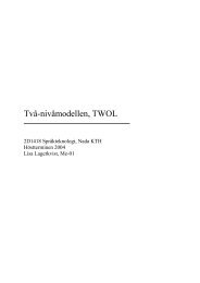
The scaled domain is seen in Figure 3.1 below.
The scaling was done as follows:
Figure 3.1. The computational Domain
˜x = x
S1
˜y = y
S1
7
(3.1)
(3.2)

where ( ˜x, ˜y) are the new coordinates of the computational domain, and S is the
scaling factor. For all sub-domains within the cell itself, the scaling factor S1 =
2.24 −6 is the radius of the nucleus. For the rectangular domain, scaling by only S1
makes its radius to be 18, which is more than four times the radius of the whole cell.
To make it graphically convenient, it is again scaled by yet another scaling factor,
in order to reduce its thickness to 0.5. Therefore, for the rectangular sub-domain in
Figure 3.1, the scaling factor is S2 = 36 × S1.
The concentration of any given species are also scaled:
˜φi = φi
C0
where C0 is the initial concentration of C in the water surrounding the cell.
3.1 The diffusion reaction model equation
(3.3)
Applying the above scaling, and combining diffusion and reaction, the general
equation for any given subdomain is given by
∂ ˜φi
∂t
= D
S ▽2 ˜φi + F˜φi
(3.4)
where ˜φ is any of the scaled species, S = S1 or S2 the scaling factor for space, and F
is the reaction term representing the rate of change of the scaled concentration due
to reaction in that subdomain. Let us again take the example of the nucleus. Then
φi is given by
∂φnu ˜ D
=
∂t S2 ▽
1
2 ˜φnu + F˜φnu
(3.5)
where φ is any of the species’ concentration present in the nucleus, namely C, U or
A, and F is the right-hand side of equations (2.6), (2.7), or (2.8), depending on the
appropriate species, and the tilde sign simply means it is normalised by the scaling
factor C0.
8

Chapter 4
Simplification of problem by means of
homogenisation
The computational domain in Figure 5.1 represents a cell whose cytoplasm is homogeneous,
rather than one which has many tiny membranes. Therefore, making
the cytoplasm homogeneous would be a wise idea. This method is know as homogenisation.
In reality, the cytoplasm is extremely densely packed with lipophilic compartments,
in the form of endoplasmic reticulii, mitochondria, etc. Such a set-up is
similar to a porous medium [7, p.5]. Therefore, the cytoplasm is a multicompartment
medium Ω consisting of two componets: the lipophilic or fatty domain Ω f
and the hydrophilic or watery domain Ωw. We then assume that the mixture is homogeneous,
i.e. a representative elementary volume (REV) taken anywhere in Ω
is identical. Let
ρ f = total volume of Ω f
total volume of Ω
(4.1)
and
total volume of Ωw
ρw = 1 − ρ f =
total volume of Ω
(4.2)
Then the following steps are taken in order to model what happens in the cytoplasm:
• finding an effective diffusion coefficient � �
Deff for the homogenised cytoplasm
• finding a new partition coefficient between the other parts of the cell and the
homogenised cytoplasm
• using the above to get the concentration of any diffusing species φ for every
point in the homogenised cytoplasm.
9

• applying an appropriate isotherm [7, pp.407,408] to get the part of the concentration
involved in reaction, since only the C within the aqueous compartment
reacts, remembering that no reaction takes place in the lipid compartments
or membranes.
4.1 Finding D eff
The diffusion path in this model is radial, directed from the cell membrane to the
nucleus. If all the membranes in the cytoplasm were oriented parallel to the diffusion
path, then D eff = Dar, where Dar is the weighted arithmetic mean diffusion
coefficient. If all the membranes in the cytoplasm were oriented perpendicular to
the diffusion path, then D eff = D ha , where D ha is the weighted harmonic mean
diffusion coefficient. In principle, in any intermediate case, Dar ≤ D eff ≤ D ha or
Dar ≥ D eff ≥ D ha [6, p.10].
4.1.1 Weighted arithmetic mean of the diffusion coefficient
The weighted arithmetic mean is obtained if all the Ω f subdomains are oriented
parallel to the diffusion path. That is, they are radially oriented in the cytoplasm. If
we take a REV containing one Ω f and one Ωw subdomain, then the rate of change
of the concentration of any species φ is given by
∂φ
∂t = ∂φ (w)
∂t + ∂φ ( f )
∂t
(4.3)
where the subscripts w and f denote the watery and fatty subdomains, respectively.
If the total volume of this REV is V , we can derive an average concentration for
it as follows:
φ = 1
Z
φdv =
v v
1
Z
φ
v
(w)dv +
v
1
Z
φ ( f
v
)dv (4.4)
v
But since φ (w) is non-zero only in Ωw, and φ ( f ) non-zero only in Ω f , (4.4) becomes
∂φ
∂t
Z
1
=
v v
Z
∂φ 1 ∂φ (w)
dv =
∂t v vw ∂t dvw + 1
Z
v v f
∂φ ( f )
∂t dv f (4.5)
where vw and v f are the volumes of the Ωw and Ω f subdomains respectively. But
the rate of change of concentration is given by (2.2). Therefore if the average
quantity ▽φ is ▽φ, and hence the average quantity ▽ 2 φ is ▽ 2 φ, then (4.5) becomes
∂φ
∂t
Z
1
= D
v eff▽ v
2φdv = 1
Z
Dw▽
v vw
2φdvw + 1
Z
D f ▽
v v f
2φdv f
10
(4.6)

and since ▽ 2 φ is constant over the REV just mentioned,
∂φ
∂t
1
=
v Deff▽2φ·v = 1
v Dw▽2φ·vw + 1
v D f ▽2φ·v f = ▽2 �
1
φ·
v Dw · vw + 1
v D �
f · v f
Applying (4.1) and (4.2), equation (4.7) becomes
and finally
∂φ
∂t = Deff▽2φ = ▽2φ · � �
ρwDw + ρ f D f
D eff = ρwDw + ρ f D f = Dar
4.1.2 Weighted harmonic mean diffusion coefficient
(4.7)
(4.8)
(4.9)
The weighted harmonic mean is obtained if all the Ω f subdomains are oriented
normal to the diffusion path. That is, they are in series with the Ωw subdomains. If
we take a REV containing one Ω f and one Ωw subdomain, then the rate of change
of the average concentration of any species φ is given by
∂φ
∂t = D · ▽2 φ (4.10)
In this case in series, ▽ 2 φ is considered separate for Ωw and Ω f . i.e
Also,
and
where ∂φ
∂t is for both Ωw and Ω f .
or
▽ 2 φ = ▽ 2 φ w + ▽ 2 φ f
▽2φw = D −1 ∂φ
w ·
∂t
▽ 2 φ f = D −1
f · ∂φ
∂t
(4.11)
(4.12)
(4.13)
Combining (4.10), (4.11), (4.12) and (4.13),
Z
1
�
▽
v v
2φw + ▽2 �
φ f dv = ∂φ
Z
1
D
∂t v vw
−1
w dvw + ∂φ
Z
1
D
∂t v v f
−1
f dv f (4.14)
Therefore
or
▽2φ = ∂φ
�
ρw · D
∂t
−1
w + ρ f · D −1
�
f
D −1
eff = ρw · D −1
w + ρ f · D −1
f
�
Deff = ρw · D −1
w + ρ f · D −1
�−1 f = Dha 11
(4.15)
(4.16)
(4.17)

4.1.3 Decision on D eff for the cytoplasm
The thin sheet-like membranes in the cytoplasm may take any orientation. Let us
now consider the 3D cell to have its membranes in any one of three orientations:
perpendicular to the diffusion path, radially oriented but vertical, or radially oriented
but horizontal. This is a perfect, un-biased orientation of the membranes,
with one-third of the membranes in each direction. Therefore one-third of the
membranes are in series with the aqueous compartment of the cytoplasm, while
two-thirds is in parallel, with respect to the diffusion path. Therefore
Deff = a · Dha + b · Dar
a + b
(4.18)
where a = 1 and b = 2. Therefore, depending on what fraction of the membranes we
think are oriented in each direction vis-a-vis the three above-mentioned directions,
a and b can be changed. However, I and the professors have thought that the unbiased
mode of orientation is most natural. Magnified 3D electron micrographs of
the cell depict such an orientation of the membranes.
Note that the diffusion coefficient along a membrane is not the same as across
it. Therefore, in calculating D ha , a different D is used than when calculating Dar.
This is implemented in the application.
4.2 Partition coefficient between homogenised cytoplasm
and other subdomains
Now that the cytoplasm has been homogenised, all its physical properties have
changed. We know the partition coefficient for the species C and U, between Ωw
and Ω f is Kp < 1. This implies that at equilibrium, Cw = Kp ·Cf and Uw = Kp ·Uf .
In other words, the concentration of either of those species in Ω f is K−1 p times
greater than in Ωw.
We now have to remember that the neighbouring subdomains to the homogeneous
cytoplasm are in Ω f : viz the outer membrane and the nuclear membrane. If
we denote the partition coefficient between this homogenised cytoplasm and any
Ω f by Kp, ˆ then Kp ˆ can be derived. With little arithmetics, we have
Kp ˆ = 1 · ρw + K−1 p · ρ f
12
K −1
p
(4.19)

4.3 Solving for concentration; Fraction of C undergoing
chemical reaction
Concentration of the species in various subdomains
Now that we have the necessary effective parameters for the homogenised cytoplasm
subdomain, the diffusion equation for this domain can be set using these
new parameters. Together with the diffusion equation of the other subdomains
which were already homogeneous and straight forward right from the beginning,
the diffusion problem of the whole domain can be solved for the concentrations C
and U which are mean concentrations for each point in the cytoplasm subdomain.
In the homogenised cytoplasm, we solve for C and U instead.
4.3.1 Reaction. Fraction of concentration affected by chemical
reaction in the cytoplasm.
Generally, reaction is as described in Chapter 2.2, but in the homogenised cytoplasm,
other considerations must be made. Since C is a weighted mean between the
Cs’ in both Ωw and Ω f , and noting that in reality chemical reaction only takes place
in the Ωw, we have to decide what fraction of C is involved in chemical reaction. In
this case we have to apply the concept of adsorption isotherm[7, pp.407,408]. An
adsorption isotherm is an expression relating the quantity of an adsorbed quantity
e.g in Ω f , to the quantity in another phase e.g in Ωw .
We shall use the equilibrium isotherm, which states that the amount of adsorbed
component is equal to the amount at equilibrium. This means that for any Ω f and
its neighbouring Ωw, we assume that
Cw = KpCf
(4.20)
This is a straight-forward isotherm, and is applicable when the phases Ω f and
Ωw in a REV are tiny enough for almost instantaneous concentration equilibrium
[7, pp.407,408] with any one of the diffusion coefficients in our problem.
The present problem is an example of this: This means that the equilibrium
isotherm is very appropriate for the present problem.
We know
C = ρwCw + ρ fCf
Applying Equations 4.20, Equation 4.21 can be written
� �
C = ρwKpCf + ρ fCf = Cf ρwKp + ρ f
and hence
13
(4.21)
(4.22)

Cf =
C
ρwCw + ρ f
and the concentration involved in chemical reaction is given by
C
Cw = KpCf = Kp
ρwCw + ρ f
14
(4.23)
(4.24)

Chapter 5
Model Implementation with FEMLAB
5.1 The Femlab Software
FEMLAB is a software package for the simulation and visualisation of partial differential
equations in one, two or three dimensions. The simulations are based
on the finite element method, abbreviated as FEM, hence the name FEMLAB. It
performs equation-based multiphysics modelling [13, p.153]. This means that we
can formulate our equations so that they actually suit our problem. The physical
domain is represented graphically in the software, and this is called the geometry,
or computational domain. If various parts of the physical domain have different
properties or phenomena, then the computational domain can be differentiated into
subdomains which will have different parameters and, maybe, equations.
The underlying mathematical structure of FEMLAB is a system of partial differential
equations (PDE)s. There are many application modes in FEMLAB, suitable
for various scientific problems. These are, so to speak, templates for defined equations
which can be modified by changing the values of some predefined parameters,
to suit the scientific problems we want to solve.
The problem at hand does not fit well into the predefined application modes.
Therefore the coefficient form of the PDE mode is used in this work. In this mode,
one physics mode[10, p.8] can handle many variables. Since there are at least two
variables in each part of the cell, this property is very useful for the present model.
5.2 The Geometry
A 2D model is sufficient for our purpose. A sector of only one-sixteenth (22.5 o ) of
the cell is used to minimise computational resources and time.
Thickness of the nucleus was used as the scaling factor. All parts of the cell are
scaled with this factor s.
15

Since the thickness of the cytoplasm and nucleus are of the order of a 1000
times that of the membranes, the graphical representation of the membranes in the
femlab Draw mode would be very thin. Therefore the triangular elements in these
thin domains would be very tiny, and thus the model would be too computationally
expensive.
One way to solve this problem would be to approximate the membranes as
simple boundaries, by a technique known as thin film approximation [4]. However,
the example in the FEMLAB manual is straightforward and involves no partition
coefficient, whereas in the present case, there is a partition coefficient because the
membrane should act as a reservoir for A and U. Of course, this is possible, but
rather inconvenient. Therefore, I chose a different approach.
The extracellular solution, as will be shown below, is 27.748 times thicker than
the nucleus whose scaled radius is 1: If we denote the scaled radius of the entire
cell by r, and that of the medium surrounding it by R, then equating the ratio of
their volumes to 168, we have
R3 = 168 (5.1)
3
r
If we then substitute r by 4 in (5.1), we find R to be 22, and therefore the scaled
thickness of the external solution alone is 22 − 4 = 18.
Therefore our computational domain consists of:
• A rectangle which represents the extracellular solution
• A thin outer arc which represents the cell membrane
• A thicker inner arc which represents the cytoplasm. The thousand of tiny
membranes in the cytoplasm are not represented in the domain because they
are handled by homogenisation.
• A thin inner arc which represents the nuclear membrane
• Finally, a thicker central circle which represents the nucleus
All the arcs are concentric with the central circle and only 22.5 o is taken, from
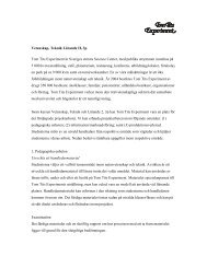
the centre of the central circle, as seen in Figure 5.1.
In the FEMLAB draw mode, the scaled domain in Figure 5.1 is drawn. The
representation of a domain in FEMLAB is called a geometry [8, p.157].
5.3 Subdomain properties, equations and constants
From the multiphysics menu, a physics is chosen depending on which subdomain,
and appropriate parameters are entered in the subdomain settings dialog box
[8, p.157] to specify the diffusion-reaction equation in that subdomain. The coefficient
form of the PDE mode is used.
16

Figure 5.1. The computational Domain
5.4 Constants and Parameters
It is most convenient to have all the variables and expressions defined in the options
menu [10, p.98] . This is so that if we want to change any coefficients or material
properties, we do not need to go to the subdomain or boundary settings and modify
these for each subdomain. We just need to modify the value by going to the options
menu. In order to know what the constants in my programme stand for, below is a
table of them:
1
5.5 Subdomains and their properties
Subdomain properties of the appropriate physics are presented in Table 5.2. The
boundaries are numbered anti-clockwise round each subdomain. We begin from
boundary 11, which is the left boundary of the extracellular water. The subscripts
indicate the subdomains. Note that for simplicity, the boundary and sub-domain
numbering in this report is not the same as in the programme.
1 The asterices (∗)in Table 5.1 indicate given data. This is the data in the programme that may be
changed by the experimenter. The rest of the entries in the table are computed by the programme.
17

constant meaning and units value
conc Initial concentration in the extracellular solution (M)∗ 1 × 10 −4
cr Fraction of C undergoing chemical reaction 347 × 10 −6
cscale Scaling factor for concentration * 1 × 10 −4
c0 Normalised Initial concentration in the medium 1.0
Dext Diffusion coefficient (D) in the extra-cellular solution � m 2 s −1� ∗ 1.3 × 10 −11
D1 D of the species in the outer membrane � m2s−1� ∗ 1 × 10−12 Effective diffusion coefficient in the cytoplasm � M · m2s−1� 3.9517 × 10−11 D2
D2T Transverse D of the species in the membrane � m 2 s −1� ∗ 1 × 10 −10
D2P Normal D of the species in the membrane � m 2 s −1� ∗ 1 × 10 −12
D3 D of the species in the nuclear membrane � m 2 s −1� ∗ 1 × 10 −12
D4 D of the species in the nucleus � −2s−1 � ∗ 1 × 10−14 D in homogenised cytoplasm if in parallel � m2s−1� 5.926 × 10−11 Dseries
D in homogenised cytoplasm if in series � m2s−1� 2.419 × 10−14 f rac1 Volume fraction of cytoplasm occupied by lipid part * 0.592593
f rac2 Volume fraction of occupied by acquous part 1 − 0.592593
G Concentration of GST (M)∗ 347 × 10−6 Dparallel
Kc Catalytic activity � M−1 · s−1� Kcc
∗
�
−1 Reaction constant of C with GST in cytoplasm = G · Kc s
660003
�
Ku Reaction constant of C with water
2.244
� s−1� ∗ 3.6 × 10−4 M Mass transfer coefficient * 1 × 10−4 n Number of cells whose volume was measured as Vn∗ 1 × 107 N Number of cells in culture * 2 × 107 num s f + sp 3
pump factor determining the rate at which B is pumped out ∗ 0.02
pk Partition coefficient between aqueous and lipid parts ∗ 1 × 10−4 pk2 Partition coefficient between membrane and homogenised cytoplasm 1 × 10 −4
Rcell Radius of cell (m) 1.92 × 10 −4
Rw Scaled radius of part of medium containing cell (m) Computed by code
s Radius of nucleus. Space scaling factor for cell (m)∗ 4.8 × 10 −6
s f Portion of membranes in cytoplasm parallel to diffusion path 2
p f Portion of membranes in cytoplasm normal to diffusion path 1
S Scaling factor of extracellular space in addition to s (m) 55.496
theta Angle of sector of circle representing the cell (radians) π 8
Tws Scaled hickness of part of medium enclosing one cell (m) Computed by code
Tw Thickness of part of medium enclosing one cell (m) Computed by code
Vw
Volume of part medium enclosing one cell � m3� 1 × 10−5 Vn Volume of n cells � m3� ∗ 3 × 10−6 Volume of one cell � m3� Computed by code
V1
Vratio Volume ratio of medium per cell Computed by code
wscale Total scaling factor for extracellular space (m) 1.3874 × 10−4 Table 5.1. Constants used in the programme
18

Physical subdomain Femlab Subdomain Variables boundaries
Water 1 C1, U1 11, 21,31, 41
Cellmembrane 2 C2, U2 32, 52,62, 72
Cytoplasm 3 C3, B3, U3 63, 83,93, 103
Nuclearmembrane 4 C4, U4 94, 114,124, 134
Nucleus 5 C5, A5, U5 125, 145,155
5.6 Initial condition
Table 5.2. Subdomains
In the sub-domamain settings mode, all initial concentrations were left at their default
value, which is 0, except that the scaled initial concentration of C in subdomain
1 was changed to c0.
5.7 Boundary conditions
In the boundary settings dialog box [12] all the exterior boundaries of the domain
were left at their default (insulation). Then choosing the appropriate physics in
FEMLAB, the default insulation was again left unchanged for species which do
not diffuse out of their subdomains. These are A and B. Then for C and U, the flux
was set according to (2.10). This is similar to separation through dialysis model
of the FEMLAB model library [3, p.213]. While all boundaries are insulated for A
and B, table 3 below sumarises the boundary conditions for C and U.
5.8 Solving
Boundary number Type
subscripts 3, 6, 9, 12 flux
remaining numbers insulation
Table 5.3. Boundary conditions for C and U
The problem was solved with the default solver parameters. It was sufficient to
solve the problem up to 250 seconds.
Solution time was only 1 minute, due to the efficiency of the programme thanks
to homogenisation.
19

5.9 Results
In Figure 5.2, concentrations inside the cytoplasm with time, are compared to the
in vitro results. The concentrations from the in vitro experiments were taken only
at a limited number of instants because it is a very difficult task. The scanty dots
represent concentrations from in vitro experiments, while the graphs are from the
simulations. It is not the actual concentrations which are plotted here, but the percentage,
where the maximum is set to 100 %. Overall, the patterns are similar. The
differences seen might be explained by that the molecular dynamics within the cell
is more complex than we assume in our model.
Figure 5.2. C, B and U in cytoplasm plotted with time
Plots of the concentration of C in the extracellular solution have been compared
to similar plots obtained experimentally by the researchers at K.I. It shows the half
life of C. Please see Figure 5.3.
Laboratory experiments showed that the half life of the substrate C in the solution
was about 63 seconds. The plot in Figure 5.2 obtained from the FEMLAB simulation
depicts a half-life of 60 seconds. This is close enough.
20

Figure 5.3. C in solution plotted against time
21

Chapter 6
Conclusion
In the laboratory, careful and tedious measurement techniques are necessary in order
to know the concentration of, for instance, A in the nucleus. Since the model
reproduces those obtained in the laboratory, it can therefore be used as a quick and
easy alternative to determine how much of the carcinogenic product A is present in
the nucleus, which is an indication of the risk of cancer. Here is a plot of the concentration
of A in the nucleus for 500 seconds. One can conclude that the model
can fulfil its aims as indicated in Chapter 1.
The results encourage us to continue developing the model alongside in vitro
experiments.In this model, the chemical reactions occur within the bulk of the aqueous
compartment of the cytoplasm. In future, a similar model is intended to be used
to solve problems where surface reactions are also included. This is the case where
the enzyme which is only present on the surface of the membranes. The present
model will, of course, facilitate the modelling of surface reaction problems, but the
homogenisation of surface reactions are very complex, and a deeper understanding
of the physics and mathematics involved in transport phenomena is needed.
22

Figure 6.1. Concentration of A in the nucleus
23

References
1. K. Sundberg, K. Dreij, A. Seidel and B. Jernstrom.Gluthion Conjugation
and DNA Adduct Formation of Dibenzol [a,1] pyrene and Benzo [a] pyrene
Diol Epoxides in V79 Cells Stably expressing Different Human Glutathione
Transferases. Chemical research in Toxicology ,2002,15, pp. 170-179
2. A. Hartmann, E. M. Golet, S. Gartiser, et al. Primary DNA Damage But Not
Mutagenicity Correlates with Ciprofloxacin Concentrations in German Hospital
Wastewaters Archives of Environmental Contamination and Toxicology,
February 1999, pp. 115 - 119.
3. COMSOL AB, Chemical Engineering Module. 2004, Stockholm, p. 213
4. COMSOL AB, Thin Film Approximation,
http://www.comsol.com/support/knowledgebase/902.php.
5. H. Fredrick, A. Barbero. Steady-state flux and lag time in stratum cornium
lipid pathway using finite element methods. Journal of pharmaceutical Sciences.
Vol 92, NO.11, November 2003, pp. 2196-2207.
6. Lars Erik Persson, Leif Persson, Nols Svanstedt and John Wyller, The Homogenization
Method, an introduction. England, Chartwell Bratt, 1993.
7. Jacob Bear and Yehuda Bachmat, Introduction to Modelling of Transport
Phenomena in Porous Media, The Netherlands, Kluwer Academic , 1990.
8. COMSOL AB, Model Library, FEMLAB3. Stockholm, 2004.
9. COMSOL AB, Chemical Engineering Module, Stockholm, 2002, pp. 2-253,
2-254.
10. COMSOL AB, FEMLAB3 Users’ Guide. Stockholm, 2004.
24

List of Abbreviations
A . . . . . . . . . . . . . . . . . . . . . . . . . . . . . . . . . . . . . . . . . . . . . . . . . . . . . . DNA adducts
B . . . . . . . . . . . . . . . . . . . . . . . . . . . . . . . . . . . . . . . . . . . . . . . . gluthione conjugates
b.c . . . . . . . . . . . . . . . . . . . . . . . . . . . . . . . . . . . . . . . . . . . . . . . . boundary condition
D . . . . . . . . . . . . . . . . . . . . . . . . . . . . . . . . . . . . . . . . . . . . . . . . diffusion coefficient
Dar . . . . . . . . . . . . . . . . . . . . . . weighted arithmetic mean diffusion coefficient
D eff . . . . . . . . . . . . . . . . . . . . . . . . . . . . . . . . . . . . . effective diffusion coefficient
D ha . . . . . . . . . . . . . . . . . . . . . . weighted harmonic mean diffusion coefficient
C . . . . . . . . . . . . . . . . . . . . . . . . . . . . . . . . . . . . . . . . . . . . . . . . . . . . . . .diol epoxides
GST . . . . . . . . . . . . . . . . . . . . . . . . . . . . . . . . . . . . . . . . . . . gluthatione transferase
K.I . . . . . . . . . . . . . . . . . . . . . . . . . . . . . . . . . . . . . . . . . . . . . . .Karolinska Institutet
Kp . . . . . . . . . . . . . . . . . . . . . . . . . . . . . . . . . . . . . . . . . . . . . . . . partition coefficient
REV . . . . . . . . . . . . . . . . . . . . . . . . . . . . . . . . . representative elementary volume
U . . . . . . . . . . . . . . . . . . . . . . . . . . . . . . . . . . . . . . . . . . . . . . . . . . . . . . . . . . . . . tetrols
25