Midterm exam with suggested answers

Economic Development 570: Midterm Exam
Professor Tybout
October 21, 2003
Please put your ID number on each page you turn in, and number you pages consecutively.
(For example, if you turn in 6 pages, number them “1 of 6,” “2 of 6,” et cetera.) Do not put
your name anywhere on the exam.
You must answer both questions in part I, and one of the two questions in part II. All
questions will receive equal weight. No extra credit will be awarded for answering all both
questions in part II.
Good luck!

Part I: Answer both of the following two questions
1) (25 minutes) We have studied four models of industrialization/modernization that explain
why multiple equilibria are possible, and why countries can get stuck in “low level traps:”
Kevin Murphy, Andrei Schiefer and Robert Vishny (MSV): “Industrialization and the Big
Push,”
Paul Krugman (K): “History versus Expectations,”
Paul Krugman and Anthony Venables (KV): “Globalization and the Inequality of
Nations,”
Dani Rodrik (R): “Coordination Failures and Government Policy: A Model with
Applications to East Asia and Eastern Europe”
a) (20 points) Each of these models involves strategic complementarities. That is, when
many agents are pursuing a given activity, the returns to pursuing that activity are
increased for other agents. Explain what form the strategic complementarities take in
each model mentioned above, and why they help to establish the possibility of
multiple equilibria.
In MSV, the strategic complementarities derive from the fact that each modern
producer is more profitable when there are other modern producers around. This is
because modern producers, when operating on a large scale, generate more income
for their employees, and thus generate more demand for output of each good. Multiple
equilibria are possible because, when no other modern sector producers are present,
no one has an incentive set up a modern facility⎯demand won’t be large enough to
make it more efficient than cottage production. On the other hand, if all of the other
producers are modern, there is sufficient demand for each product to make modern
production more profitable than cottage production.
In K, the wage rate depends positively on the fraction of the labor force in the modern
sector, but the strategic complementarities aren’t spelled out in detail. This
specification implies external economies at the sector level, due perhaps to
agglomeration economies, richer menus of intermediate goods (as in R), or the
sharing of specialized knowledge. Multiple transition paths are possible because one’s
beliefs about the behavior of other suppliers of factors influence one’s own behavior.
More specifically, if one expects everyone else to move toward modern sector
production, one is inclined to do so as well. However, unlike in MSV, the scope for
multiple equilibria hinges upon the importance of adjustment costs, when create an
incentive to move slowly.
In KV, the strategic complementarities come from the fact that the location of other
producers determines the payoff to one’s own firm at each possible location. This is
because being close to other firms and their workers increases their demand for your

product (transportation is costs). On the other hand, concentration of production in a
limited geographic area drives up the cost of employees. When transport costs are
moderate, multiple equilibria are possible⎯one with manufacturing production
consolidated in a single region and with manufacturing production spread evenly
across all regions. In the former case, with consolidated production, the neglected
region has no demand for manufactured inputs and its workers have little income, so it
is a relatively unattractive place to locate. In the latter case, a movement toward
consolidation would generate more local demand for the marginal firm, but the gains
from this would be more than offset by the loss in demand due to extra transport costs
when servicing customers abroad.
In R, strategic complementarities result from the fact that the high-tech sector uses
non-traded intermediate inputs, and the larger the menu of these intermediate inputs,
the more efficiently it produces. There are scale economies in intermediate goods
production, so the more demand there is for intermediate inputs, the larger the
available menu of these goods. Hence when few high-tech producers are active, the
menu of goods is small, and the return to high-tech production is low, so the economy
tends toward low-tech production. On the other hand, when many high-tech producers
are active, there are many intermediate goods available and the return to high-tech
production is high, so the economy gravitates toward high-tech production.
b) (13 points) Suppose a country is stuck in a low-level trap, and its economic minister
asks you how to escape. Are there policies that would tend to push the country out of
low-level equilibrium, regardless of which model applies? Are there policies that
would work only under the assumptions of some of the models?
Increased demand for the high-tech/modern good will generally tend to push an
economy toward that type of production. In each context this might take the form of a
subsidy, or at least a guaranteed minimum profit rate (which wouldn’t actually cost
the government money if it successfully moved the economy to a modern equilibrium).
Some policy implications are specific to the model, however. For example, if transport
costs are small, simply opening the MSV model to trade would de-link modern sector
profitability from size of the modern sector. In the context of K, subsidies to workers
for retraining might reduce the relative importance of history, and combined with
guaranteed minimum earnings in the modern sector, might bump the economy to a
modern sector equilibrium. In KV, trade protection would force the emergence of
domestic manufacturing; it is possible that after accomplishing this the economy
would become a global manufacturing sector, or at least avoid specializing in
agriculture, even if the protection is subsequently removed. Finally, in the context of
the R model, subsidies to capital formation or the removal of barriers to international
capital mobility may reduce the wage-rental ratio sufficiently that high-tech equilibria
dominate. Minimum wages might even accomplish the same thing.

2) (25 minutes) The per capita income of Malsuerte has remained close to subsistence for
the past 50 years. The Malsuertian government is convinced that the problem is a poor
schooling system, so it has decided to deliver heavily subsidized primary and secondary
education to all school-age children.
a) (18 points) Drawing on the models of Robert Lucas (“On the Mechanics of Economic
Development”), and Gary Becker, Kevin Murphy and Robert Tamura (“Human
Capital, Fertility and Economic Growth”), carefully explain why this policy might lead
to higher per capita income growth.
In the Lucas model, there are external returns to human capital, so without subsidies,
too little gets produced in the market equilibrium. Further, the rate of growth in total
factor productivity depends upon the rate of human capital accumulation, so when
agents react to subsidized education by investing more in secondary education, the
rates of productivity and output growth should increase. Of course, this presumes that
the Lucas representation of human capital accumulation, which presumes that the
growth rate in human capital is proportional to the faction of the time individuals
spend schooling, is correct.
In the BMT model, parents with low education levels maximize their utility by having
large numbers of uneducated children. This is because (1) they are not very efficient at
teaching their children, and (2) they are earning low wages, so the time costs of child
rearing are relatively low. A subsidy to education may shift the balance in favor of
small numbers of educated children. Further, it may result in steady state growth if the
time costs of having children are sufficiently high, parents are relatively productive at
endowing their children with education (given their own human capital level), and/or
the marginal utility parents derive from additional children falls rapidly with n.
b) (15 points) Suppose the Malsuertian economy is actually stuck in a low level trap of
the type described by Dani Rodrik (“Coordination Failures and Government Policy: A
Model with Applications to East Asia and Eastern Europe”). Will adding to the human
capital stock help, hurt, or do nothing? Carefully explain. You may find it useful to
draw a graph.
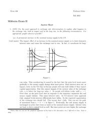
This policy shock can be analyzed using the graph below.

w
θ ( w,
r)
= 1
( r , wλ(
h)
c(
z)
) π
φ =
r
Here the function θ ( w,
r)
shows the cost of producing one unit of low-tech output
when wages and rental rates are w and r, respectively. Similarly, the function
⎛
−1
⎞
⎜
−1
⎟
φ
σ
⎜r , wλ(
h)
c(
z)
n ⎟ gives the cost of producing one unit of high-tech output at these
⎝
⎠
factor prices when the human capital stock is h and the number of (non-traded)
intermediate varieties produced domestically is n. In equilibrium, if only one type of
good is produced and factor markets clear, the slope of that good’s isocost contour
must match the capital labor ratio, which is depicted as a negatively sloped line
segment. If the economy specializes in one good, it will choose the good that generates
the larger factor payments. The outer hull of the two unit cost functions shows which
product this will be and the associated factor prices, when the prices of low-tech and
high-tech goods are 1 and π , respectively, and the capital-labor ratio is given by the
negatively sloped line segments. Low-tech equilibria are sustainable if specialization
in the low-tech product generates more factor income than would be generated by one
high-tech producer and all other resources devoted to low-tech production (see
figure). Since the function λ(h) c(
z)
gives the unit labor requirements for intermediate
⎛
−1
⎞
⎜
⎟
production, and λ '(
h)
< 0 , the φ r wλ( h)
c(
z)
nσ
−1
⎜ ,
⎟ = π contour shifts outward when
⎝
⎠
the human capital stock increases. Thus, if subsidies to human capital accumulation
increase h, they may do nothing to the equilibrium (small shift), lead to a diversified
economy (shift to dotted isocost line), or lead to specialization in high tech goods (shift
to heavy dotted line). Although the graph does not reveal it, n adjusts if the nature of
the equilibrium changes. Not also that the latter two shocks eliminate the low- tech
equilibrium, so that coordination is no longer an issue.

Part II: Answer either of the following two questions
3) (25 minutes) Some economists have argued that unusually rapid factor accumulation has
driven growth among the countries that have successfully developed during the past 30
years. (See, for example, Alwyn Young, “The Tyranny of Numbers, . . .” and Gregory
Mankiw, David Romer and David Weil, “A Contribution to the Empirics of Economic
Growth.”) Others have argued that productivity growth has been the key to their
success⎯perhaps reflecting successful escape from a poverty trap. (See, for example,
Peter Kenow and Andrés Rodriguez-Clare, “Has the Neoclassical Revolution Gone too
Far?”)
a) Describe and critically evaluate the methodologies that these authors have used to
arrive at their conclusions.
Young uses a total factor productivity decomposition based on the total differential of
a neoclassical production function:
∆ ln( A ) = ∆ ln( Y
t
t
/ L ) −
t
[ s ∆ ln( K / L )]
K
t
t
⎡
− ⎢s
⎢⎣
K
⎛ K
∆ ln⎜
⎝ K
*
t
t
⎞
⎟
+ s
⎠
L
*
⎛ Lt
∆ ln⎜
⎝ Lt
⎞⎤
⎟
⎥
⎠⎥⎦
Here A represents the productivity level, s ’s are factor shares in total cost, and
variables with asterisks are quality adjusted input measures. The expression states
that growth in output per worker is due to (1) increases in the capital labor ratio, (2)
increases in the quality of inputs, or (3) growth in total factor productivity. Applying
this decomposition to data from the gang of 4 countries, he finds that their productivity
growth performance, while solid, was not extraordinary. Hence he concludes that
these countries grew exceptionally rapidly simply because they accumulated factors
and improved factors at an exceptional pace.
Easterly and Levine complain that Young’s study would attribute growth to factor
accumulation even if it were induced by productivity growth. So this study may not be
the best way to sort out whether productivity growth is key. To get around this
critique, Mankiw, Romer and Weil assume a Cobb-Douglas technology that includes
labor, human capital, and physical capital: Y = C + I
Y ⎛
which implies = A⎜
L ⎝
K
Y
⎞
⎟
⎠
1
α
−α−β
⎛
⎜
⎝
H
Y
⎞
⎟
⎠
1
β
−α−β
α β 1−α−β
K + I H = K H (AL) ,
= AX . Then using the steady state savings
rates in physical and human capital they obtain
K I K / Y
= and
H I H / Y
= ,
Y g + δ + n Y g + δ + n
which substituted into the previous expression yield an equation for per worker
income in terms of investment rates in physical and human capital when all lower-case
and Greek characters are treated as parameters. This expression explains a large
fraction (74 percent) of the cross-country variation in per worker income, so they
conclude that factor accumulation is the key to living standards. Kenow and

Rodriguez-Clare question this conclusion on two counts: they complain that MRW
didn’t include primary education in their measure of human capital investment, and
they say that the technology which converts output to physical capital isn’t the same as
the technology that converts output to human capital. Re-doing the exercise, they
reduce explain variation to 40 percent, and argue that productivity differences are an
important part of the recipe for success.
b) Does the debate boil down to disagreement about whether savings causes growth or
responds to it? Explain.
4) (25 minutes) Below are some commonly held beliefs about the typical transition from
extreme poverty to industrialized status. Critically evaluate the empirical evidence on each
statement, and indicate whether you feel it is valid. Pay attention to empirical
methodologies.
a) (8 points) Income distribution becomes relatively less equal before it improves.
The early literature on inequality and development found this pattern, but it was based
on cross-sectional analysis of poor data. It largely reflected the fact that Latin
American countries were in the middle of the per capita income range and they had
relatively unequal (measured) income distributions. More recent studies that follow
countries through time (pooling countries and including country dummy variables)
tend not to find any relationship between per capita income and growth; a few even
find that growth makes the distribution more equal.
b) (8 points) Countries starting from low per capita income levels grow relatively rapidly,
then slow down.
Prior to entering the “intensive growth” phase, many countries spend years in low
level poverty traps. When they begin to develop, growth accelerates, and after the
transition period, they settle down into long-run positive growth. It is also true that,
looking across countries that span a wide range of income levels, growth regressions
usually find a negative relationship between initial per capita GDP and subsequent
growth. However, this at least partly reflects the fact that initial per capita GDP
figures negatively into per capita growth by construction.
c) (8 points) Falling fertility rates typically precede the “intensive growth” phase, during
which per capita output growth accelerates.
No, a country enters the intensive growth phase, morbidity falls first as health
conditions improve. The fertility rate starts to fall later, so there is an early transition
period during which population growth accelerates.

d) (8 points) Despite growth in per capita incomes, poor countries have been getting
poorer relative to rich countries.
As Pritchett documents, the less developed countries have been growing more slowly
that the advanced capitalist countries during the past century. Many of the poor
countries that have experienced the lowest growth rates haven’t kept good data, so the
contrast in performance is probably less dramatic than it would be if it were based on
the full sample of countries.