Synthetic Inflow Condition for Large Eddy Simulation (Synthetic - KTH

Synthetic Inflow Condition
for Large Eddy Simulation
(Synthetic Eddy Method)
EVELYN OTERO
Master of Science Thesis
Stockholm, Sweden 2009

Synthetic Inflow Condition
for Large Eddy Simulation
(Synthetic Eddy Method)
EVELYN OTERO
Master’s Thesis in Numerical Analysis (30 ECTS credits)
at the Scientific Computing International Master Program
Royal Institute of Technology year 2009
Supervisor at CSC was Jesper Oppelstrup
Examiner was Michael Hanke
TRITA-CSC-E 2009:112
ISRN-KTH/CSC/E--09/112--SE
ISSN-1653-5715
Royal Institute of Technology
School of Computer Science and Communication
KTH CSC
SE-100 44 Stockholm, Sweden
URL: www.csc.kth.se

Abstract
Today, whereas aeronautical CFD applications are mainly
based on Reynolds Average Navier-Stokes modeling, Large
Eddy Simulation (L.E.S.) is becoming more used for some
of them. LES needs the instantaneous inlet velocity as turbulent
inflow boundary conditions which motivates the implementation
and validation of a synthetic turbulent inflow
condition for LES. The so called "Synthetic Eddy Method"
(SEM), which is a stochastic algorithm that generates instantaneous
velocity, has been studied and validated in homogeneous
isotropic turbulence (HIT).A parametric study
was conducted in order to extend the SEM to channel flow
and comparisons with other boundary conditions such as
the periodic LES were carried out.

Referat
Syntetiska virvlar som inflödesvillkor för
Large Eddy - simulering
Large Eddy - Simuleringar (LES) blir allt vanligare som
ersättare för Reynolds-Averaged Navier-Stokes beräkningar
för extern och intern aerodynamik. LES-modeller behöver
ett turbulent inflöde. I detta arbete studeras Synthetic Eddymetoden,
som med stokastisk metod genererar ögonblickliga
hastighetsfält. Metoden har implementerats i en industriell
strömningslösare (elsA) och validerats på fall med
homogen isotrop turbulens och utvidgats till kanalströmning.
SEM jämförs med andra metoder som periodisk LES
som "återanvänderden strömning som lämnar området.

Acknowledgments
Firstly I would want to thank my supervisor at CERFACS Jean-François Boussuge
who followed carefully the progression and quality of the work through a defined
schedule and was always available for any assistance. Moreover I wanted to express
my grateful to Hugues Deniau, Marc Montagnac and Guillaume Puigt for
their regular support regarding the implementation inside the elsA code or technical
problems. Then I appreciated the work atmosphere at CERFACS, namely, very
professional and international through many seminars, as well as very convivial and
friendly. Finally I thank my professors from KTH, Michael Hanke and my supervisor,
Jesper Oppelstrup, as well as Ulrich Rüde, from the University of Erlangen,
to have allowed me to realize my master’s thesis abroad during the double degree
program, being always motivating and available for any advice.

Contents
1 Introduction 1
2 Background 3
2.1 LES Governing Equations . . . . . . . . . . . . . . . . . . . . . . . . 3
2.2 Sub-Grid Scale Model . . . . . . . . . . . . . . . . . . . . . . . . . . 5
2.2.1 Sub-grid viscosity concept . . . . . . . . . . . . . . . . . . . . 5
2.2.2 Smagorinsky model . . . . . . . . . . . . . . . . . . . . . . . . 6
2.2.3 WALE (Wall Adapting Local Eddy-Viscosity) model . . . . . 7
2.3 Numerical Method . . . . . . . . . . . . . . . . . . . . . . . . . . . . 8
2.3.1 Flux computation . . . . . . . . . . . . . . . . . . . . . . . . 9
2.3.2 Time integration . . . . . . . . . . . . . . . . . . . . . . . . . 11
2.4 Generation of Inflow Boundary Conditions for LES . . . . . . . . . . 13
2.4.1 Introduction . . . . . . . . . . . . . . . . . . . . . . . . . . . 13
2.4.2 Recycling Methods . . . . . . . . . . . . . . . . . . . . . . . . 13
2.4.3 Synthetic Turbulence . . . . . . . . . . . . . . . . . . . . . . . 16
3 The Synthetic Eddy Method 21
3.1 Principle: SEM basic equations . . . . . . . . . . . . . . . . . . . . . 21
3.1.1 Definition of the box of eddies . . . . . . . . . . . . . . . . . 22
3.1.2 Computation of the velocity signal . . . . . . . . . . . . . . . 23
3.1.3 Convection of the population of eddies . . . . . . . . . . . . . 23
3.1.4 Regeneration of the eddies out of the box . . . . . . . . . . . 24
3.1.5 Synthesis . . . . . . . . . . . . . . . . . . . . . . . . . . . . . 24
3.2 Signal characteristics . . . . . . . . . . . . . . . . . . . . . . . . . . . 25
3.2.1 A stationary ergodic process . . . . . . . . . . . . . . . . . . 25
3.2.2 Mean flow and Reynolds stresses . . . . . . . . . . . . . . . . 25
3.2.3 Higher order statistics . . . . . . . . . . . . . . . . . . . . . . 28
4 Results 31
4.1 Homogeneous Isotropic Turbulence (HIT) . . . . . . . . . . . . . . . 31
4.1.1 Definition . . . . . . . . . . . . . . . . . . . . . . . . . . . . . 31
4.1.2 Simulation setup and parameters . . . . . . . . . . . . . . . . 32
4.1.3 Statistics . . . . . . . . . . . . . . . . . . . . . . . . . . . . . 33

4.1.4 Parameters influence: Spatial and temporal analysis . . . . . 34
4.1.5 Transition to a Non-HIT . . . . . . . . . . . . . . . . . . . . . 40
4.2 Channel Flow Computations . . . . . . . . . . . . . . . . . . . . . . 41
4.2.1 Spatially Developing Channel Flow . . . . . . . . . . . . . . . 41
4.2.2 Periodic Channel Flow . . . . . . . . . . . . . . . . . . . . . . 47
4.2.3 Statistics . . . . . . . . . . . . . . . . . . . . . . . . . . . . . 48
5 Discussion 51
Bibliography 53

Chapter 1
Introduction
Turbulent fluid flow simulation have shown to have a relevant aspect in some industrial
applications, for instance in aeronautics. In fact we can observe this phenomena
in the flows around aircrafts, in the mixing of fuel and air in the engines. Being
the cause of several problems like noise, instability due to turbulent vortices on the
surface of the aircraft, an accurate simulation of turbulent flow is extremely necessary
for a well operating system, improving design processes for cheaper and faster
aircrafts constructions.
For this purpose there are different simulation methods depending on the area
considered (level of turbulence) or the kind of application we are interested in.
Only for low Reynolds numbers and simple geometries is a Direct Numerical Simulation
(DNS) of the Navier-Stokes equations feasible without any turbulence model.
For high Reynolds numbers, Reynolds-averaged Navier-Stokes (RANS) simulations
offer another alternative, that resolves only the mean motion and relies on a turbulence
model to represent the turbulence. Between RANS and DNS lies Large-Eddy
Simulation (LES), which resolves large eddies while the smaller ones are modeled.
This method is becoming widely used in some industrial applications and
this project focuses on LES and specification of realistic inlet boundary conditions
which play a major role in the computation. Thus the project will implement and
validate a turbulent inflow condition for LES. This condition should be able to
represent accurately the turbulence characteristics. We study the "Synthetic Eddy
Method"(SEM), which is a stochastic algorithm that generates instantaneous velocity.
Hence, this report will focus on this method, starting from an introduction to
the LES theory, followed by the presentation of the Synthetic Eddy Method, and
finishing by its implementation and results analysis comparing it to another method
as the periodic LES.
1

Chapter 2
Background
Large-eddy simulations (LESs) of turbulent flows are actually extremely powerful
techniques consisting in the elimination of scales smaller than some scale ∆x by a
proper low-pass filtering [26].
LES comes from the meteorological community with the pioneering work of
Smagorinsky [43]. The first application in an engineering flow was performed by
Deardorff [5], for a fully developed channel flow and since the 1990s the number of
applications and flow conditions treated with LES has kept growing. In fact LES
has contributed to a blooming industrial development in the aerodynamics of cars,
trains, and planes; propulsion, turbo-machinery; thermal hydraulics; acoustics; and
combustion as well as in many applications in meteorology.
The Kolmogorov theory defines the small scales in the inertial and dissipative
range as having a universal behavior and being parametrizable solely by the energy
transfer rate entering the cascade. Large-eddy simulation (LES) will then pose a
very difficult theoretical problem of subgrid-scale modeling, namely, how to account
for small-scale dynamics in the large-scale motion equations. Hence the aim of using
LES is to reduce the considerable computational cost of DNS simulating only in a
direct way large scales of turbulence and modeling the smaller scales. For wall flows
at high Reynolds numbers, LES and proper computational mesh refinement can
save 99% of the effort devoted to resolving scales in the dissipation range (Pope,[38])
compared to DNS of isotropic turbulence at moderate Reynolds number.
The mathematical expressions related will be developed in this section as well
as the different models for the small eddy scales. Moreover the numerical method
used in the elsA code (cf. chapter 4.2) will be exposed followed by an introduction
to the different methods regarding the generation of Inflow Boundary Conditions
for LES.
2.1 LES Governing Equations
In this section, based on the Ref. [18], the LES governing equations of the motion
of the flows for averaged and filtered quantities are derived and later details of the
3

CHAPTER 2. BACKGROUND
turbulence models used to close the equations are provided. Although the software
elsA solves the compressible Navier-Stokes equation, we will restrict ourselves to
the simulation of incompressible flows where the mass density ρ and the dynamic
viscosity µ are constant. In this case, the Navier-Stokes equations governing the
evolution of the velocity u and pressure p of the fluid read
ρ ∂u
∂t
+ ∇.(ρu ⊗ u) = −∇p + ∇.σ (2.1)
∇.u = 0 (2.2)
The viscous stress tensor is σ = 2µS for a Newtonian fluid where
is the strain rate tensor.
S = 1
2 (∇u + (∇u)T ) (2.3)
However since the direct numerical simulation of the above Navier-Stokes equations
requires an extreme computational cost due to the several scales involved, a
smoothing operator has to be applied to the exact solution u of the Navier-Stokes
equations. The complexity of the system to be solved will thus be reduced.
Assuming that the LES spatial filter and the derivative operators commute,
governing equations for the filtered/averaged quantities u and p can then be derived,
where u corresponds to the LES averaging operators
ρ ∂u
∂t
+ ∇.(ρu ⊗ u) = −∇p + ∇.(σ + τ) (2.4)
∇.u = 0 (2.5)
And the subgrid-scale stress tensor is τ = −ρ(u ⊗ u − u ⊗ u)
Hence the LES representations of the flow field are seen as two levels of description
of the exact solution u of the Navier-Stokes equations.
Labourasse and Sagaut [20] defined the LES spatial filtering operator (see Eq.
(2.6)) in the general framework of multilevel methods relying on different scale
separation operators.
In fact the separation of large scales and small scales is done via a low-pass
filtering operation, which is defined as a convolution product
� +∞
u = G ⋆ u = u(y)G△ (x − y)dy (2.6)
−∞
4

2.2. SUB-GRID SCALE MODEL
where G △ is the convolution kernel characteristic of the filter used and △ is the
associated cutoff scale.
By the convolution product of the Eq. (2.6), motions smaller than the cutoff
scale are removed, thus the velocity u becomes smoother.
As noted before, applying this filter to the Navier-Stokes equations results in
a new set of equations for the filtered velocity u (see Eq. (2.4) and (2.5) ). It
differs from the original Navier-Stokes equations by the presence of the subgridscale
stresses τ = −ρ(u ⊗ u − u ⊗ u) which needs to be modeled as a function of
known averaged quantities in order to close the set of equations.
The most popular model for the subgrid-scale stresses are eddy viscosity models,
such as the model proposed by Smagorinsky [43] and the WALE (Wall Adapting
Local Eddy-Viscosity)[13] model presented as follows.
2.2 Sub-Grid Scale Model
The effect of the small-scale turbulence on the resolved scales is modeled using a
subgrid scale (SGS) model. The SGS model commonly employs information from
the smallest resolved scales as the basis for modeling the stresses of the unresolved
scales.
2.2.1 Sub-grid viscosity concept
An analogy with the kinetic theory of gases has been used to model the direct cascade
of energy towards subgrid-scales. We assume that the mechanism of energy
transfer of the resolved scales towards subgrid-scales can be represented by a diffusion
term using a subgrid viscosity µsm. A Boussinesq formulation is used where
the deviatoric part of the subgrid constraints tensor is linked to the deformation
tensor of the resolved field by:
τ t ij − 1
3 τ t kkδij = −2µSmTij
Where Tij is the deviatoric part of the deformation tensor:
(2.7)
Tij = Sij − 1
3 Skkδij, (2.8)
The subgrid viscosity µsm has to be modeled. We consider in this study that
τ t kk is absorbed by the pressure term. We redefine then a modified pressure ΘP and
a modified temperature ΘT :
ΘP = P − 1
3 τ t kk
5
(2.9)

ΘT = ˜ T − 1
The state equation is written [10]:
2ρCυ
ΘP ≈ ρRΘT
τ t kk
CHAPTER 2. BACKGROUND
(2.10)
(2.11)
The subgrid viscosity µsm with a scale of length l0 and a time scale t0 characteristics
of the subgrid quantities. The models will have to determine these characteristic
scales and here we define two of them, the Smagorinsky and the WALE model which
is used for the computations of this project.
2.2.2 Smagorinsky model
This is an old model, at the origin of other important models. It is based in the
resolved scales and uses a similar approach to the model of Prandtl mixture length.
If we assume that the cutoff scale △c imposed by the filter is representative of the
subgrid modes, then we obtain the length scale l0 :
l0 = Cs△c
(2.12)
A time scale is defined by assumption of local equilibrium between the kinetic
energy production rate, the dissipation energy rate by viscosity in internal energy
and the kinetic energy flux through the cutoff imposed by the filter:
1
t0
= (2SijSij) 1/2
(2.13)
The eddy viscosity of the subgrid structures ({νsm}) is proportional to the product
of a length by a velocity, thus it is written
νsm = C 2 s ∆ 2�
2SijSij
with Cs the constant of the model to determine and (here)
Sij = 1
�
∂Ui
+
2 ∂xj
∂Uj
�
∂xi
(2.14)
(2.15)
If we assume the energetic cascade of Kolmogorov, the constant Cs can be
evaluated (Ref.[23]) in a way such that the subgrid dissipation is equivalent to
the unresolved scales dissipation:
6

2.2. SUB-GRID SCALE MODEL
Cs = 1
π
� �−3/4 3Ck
≈ 0.18 (2.16)
2
where Ck = 1.4 is the Kolomogorov constant. In practice, this model is known to
be too dissipative for flows where an average shear is present such as boundary layer.
Moreover, it cannot predict [10] dynamics of weakly turbulent flows or transitional
flows.
2.2.3 WALE (Wall Adapting Local Eddy-Viscosity) model
The WALE model (Wall Adapting Local Eddy-Viscosity) is based on the Smagorinsky
approach where the time scale, characteristic of the subgrid scales, is build with
the deformation tensor {Sij} and the rotation tensor {Ωij}. This new formulation
can take into account the turbulent regions where the vorticity is bigger then the
deformation rate and it can also provide, without using any damping function, the
good behavior of the subgrid viscosity νsm in the proximity to the walls. In fact it
has been developed as a solution to the main problems coming from the Smagorinsky
model, which are [7]:
• The incapacity to predict the laminar-turbulent transition
• A too important subgrid dissipation (phenomenon changing with the distance
to the wall)
Nicoud and Ducros [7] proposed the following subgrid viscosity definition:
νsm = Cm△ 2 c{OP }( −→ x , t) (2.17)
Where Cm is the constant of the model, ∆c the characteristic length scale of the
subgrid structures and OP a spatial and temporal operator defined from the resolved
field. The Smagorinsky model is obtained for setting {OP } = (2{Sij}{Sij}) 1/2 .
However, and in accordance to the recent observations [10], this operator OP is not
only linked to the deformation rate. The WALE model defines νsm as function of
the deformation rate and of the rotation rate as:
with
S d ij = 1
2
νsm = C 2 ω△ 2
(S d ij Sd ij )3/2
({Sij}{Sij}) 5/2 + (S d ij Sd ij )5/4
⎛�
�2 � �2
∂{Ui} ∂{Uj}
⎝ +
∂xj ∂xi
⎞
⎠ − 1
�
∂{Uk}
3 ∂xk
7
�2
δij
(2.18)
(2.19)

and
2.3 Numerical Method
CHAPTER 2. BACKGROUND
C 2 m ≈ 10.6C 2 s ≈ 0.58 (2.20)
Among the important number of numerical methods simulating the viscous fluid,
some of them will be presented on this section taken from the Ref.[6]. But firstly
we need to define the hypotheses used for external aerodynamics which are the
followings:
• The air is considered as being a perfect gas
• The kinetic viscosity of the air depends only on the temperature. Exemple:
the law of Sutherland
µ
µ∞
� �3/2 T T∞ + S1
=
T∞ T + S1
(2.21)
Where T is the temperature, µ∞ the kinetic viscosity for the reference temperature
T∞ and S1 a constant (110 · 3 ž for air).
• The conductive heat flux −→ q is given by the Fourier law
−→ q = −λ −−→
gradT (2.22)
With these hypotheses, the Navier-Stokes equations are written:
∂ −→ W
∂t
With −→ ⎜
W the vector of the conservative variables ⎜
⎝
+ divF = 0 (2.23)
⎛
ρ
ρu
ρv
ρw
ρE
⎞
⎟ where E is the kinetic
⎟
⎠
energy, F the flux matrice, F equals to F = f − fv where f is the matrice of the
convectiv flux and fv is the matrix of the viscous flux.
8

2.3. NUMERICAL METHOD
�
∂Ui
with τ = µ xj
⎛
⎜
f = ⎜
⎝
⎛
⎜
fv = ⎜
⎝
�
∂Uj
+ xi
ρu ρv ρw
ρu 2 + p ρuv ρuw
ρuv ρv 2 + p ρvw
ρuw ρvw ρw 2 + p
u(ρE + p) v(ρE + p) w(ρE + p)
0 0 0
τxx τxy τxz
τxy τyy τyz
τxz τyy τzz
(τU)x − qx (τU)y − qy (τU)z − qz
− 2
3
⎞
⎟
⎠
⎞
⎟
⎠
µ ∂Uk
∂xk δij = 2µS − 2
3 µdiv(� U)I the shear constraints
tensor and −→ q the vector of the conductive heat flux computed with the Fourier law.
In the context of a finite volume approach , we integrate the Eq.(2.23) over a
control volume Ω. The problem to solve becomes:
�
Ω
∂ −→ W
∂t
dV +
�
F .�ndS = 0
∂Ω
(2.24)
Where �n is the normal vector to the surface of the control volume.
In the code of computation of elsA, it has been decided to decouple the time integration
and the spatial discretization, therefore we can choose the time integration
scheme independently of the spatial discretization method.
In order to solve numerically these non-stationary flow problems, we have to
treat the following points:
1. How to compute the flux (computation of �
the spatial discretization
2. The type of time integration
∂Ω
F .�ndS) which corresponds to
3. The linearization (if it’s necessary: in the implicit case for example)
4. A method of linear system resolution
In this section the two first points will be treated, and more details can be found
on the Ref. [6].
2.3.1 Flux computation
2.3.1.1 Convective flux computation
This section presents two methods of computation of convective flux. The term
�
�
�
∂Ω F .�ndS of the Eq.(2.24) can be decomposed as ∂Ω f.ndS − ∂Ω fv.�ndS but we
will focus on the computation of the first term .
9

Scheme of Jameson with artificial dissipation
CHAPTER 2. BACKGROUND
Since this scheme is based on a central approximation of flux, the resultant numerical
scheme is stabilized by artificial dissipation. Moreover structured grid will be
considered and will be presented in 2D as following:
Figure 2.1. Conventions
The term �
�
∂Ω f.�ndS on the cell (i, j) can be then decomposed into: (i+1/2,j) f . . . �ndS+
�
(i−1/2,j)
f . . . �ndS + �
(i,j+1/2)
The numerical flows −→ F i+1/2,j = �
ten:
�
f . . . �ndS + (i,j−1/2) f . . . �ndS
(i+1/2,j)
�F i+1/2 = f i+1/2.�s i+1/2 − � d i+1/2
f.�ndS for the central scheme are writ-
(2.25)
with f i+1/2 the matrix of the convective flux computed on the interface(i+1/2, j)
of the control volume (i, j), �s i+1/2 the surface vector (equal to the normal vector of
the interface multiplied by its surface) and � d i+1/2 a dissipation term.
Roe scheme
The numerical flux for the scheme of Roe is:
−→
F i+1/2 = 1
�
2 f( −→ W L
i+1/2) + f( −→ W R
�
i+1/2) . � (s) i+1/2
− 1
�
�
�
2 �A(−→ W L
i+1/2, −→ W R
�
�
�
i+1/2�
(−→ W R
i+1/2 − −→ W L
i+1/2) (2.26)
Where A is the matrix of Roe and −→ W L
i+1/2 and −→ W R
i+1/2 are the values of the
conservative variables on the interfaces. These values are interpolated by noncentral
schemes of order more or less big depending on the desired precision.
10

2.3. NUMERICAL METHOD
2.3.1.2 Computation of the Diffusive flux
The computation of the diffusive flux F is always done in elsA [8](para.3.5.2) with
a central approach.
2.3.1.3 Conclusion
Thus after the application of the spatial discretization following the previous methods,
the Eq.(2.24) becomes:
With V (i,j) the volume of the cell, and
d �
−→
�
V (i,j) W (i,j) +
dt
−→ R (i,j) = 0 (2.27)
−→ R (i,j) = −→ F (i+1/2,j) − −→ F (i−1/2,j) + −→ F (i,j+1/2) − −→ F (i,j−1/2)
−→ F v(i+1/2,j) − −→ F v(i−1/2,j) + −→ F v(i,j+1/2) − −→ F v(i,j−1/2)
(2.28)
Which corresponds to the set of convective and diffusive flux over the control
volume.
2.3.2 Time integration
2.3.2.1 Explicit method : Runge Kutta exemple
In order to integrate in time the Eq.(2.27), a Runge Kutta scheme can be applied
as the following, for a 4 steps case:
−→
W (1) = −→ W n − α1 ∆t
V
−→
W (2) = −→ W n − α2 ∆t
V
−→
W (3) = −→ W n − α3 ∆t
V
−→
W (4) = −→ W n − α4 ∆t
V
−→
W n+1 = U (4)
−→ R( −→ W n )
−→ R( −→ W (1) )
−→ R( −→ W (2) )
−→ R( −→ W (3) )
Explicit methods have conditional stability. In fact using this time integration
and a second order central scheme for the spatial discretization for the model
= 0, the theoretic criteria of linear stability requires a Courant-
equation ∂u
∂t
+ a ∂u
∂x
Friedrichs-Lewy number as CF L = a∆t
∆x ≤ 2√ 2(cf.[14]) but a stricter limit exits
for the boundary layer because ∆x becomes very small. This corresponds to the
viscous time step limit : ∆t ≤ C.∆x 2 . For non-stationary simulations of viscous
fluid, the size of the cells can become very small which means that the limitation
in the integration step imposed by the CFL condition can sometimes require an
important computational cost or can even cause an impossible simulation.
11

2.3.2.2 Implicit method
CHAPTER 2. BACKGROUND
For the time integration, we use multi-step linear schemes. If we use a one step
scheme (Backward Euler scheme), the Eq.(2.27) becomes:
V
−→
W n+1 − −→ W n
∆t
+ −→ R( −→ W n+1 ) = 0 (2.29)
And the linearization of the residual at the time n+1 gives
Thus the Eq.(2.29) becomes:
−→ R n+1 = −→ R n + ∂ −→ R
∂W |n ∆ −→ W n + θ(∆t 2 ) (2.30)
�
V
I +
△t
which can be more linearized (cf. [6])
−→
∂R
−−→
∂W |n
�
∆ −→ W n = −R( −→ W n ) (2.31)
2.3.2.3 Dual time step or Dual time Stepping (DTS)
DTS is another temporal integration method, which consist in using a fictive time
step solving an equivalent problem pseudo-stationary. The non stationary problem
at the time (n + 1)dt leads to the resolution of the following equation:
−→ R ∗ ( −→ W n+1 ) =
� −→ �n+1 dV W
+
dt
−→ R( −→ W n+1 ) = 0 (2.32)
Three advantages concern this method: Firstly the approximation of the temporal
derivative can be realized for any order (cf. [3]). The precision in time can
be thus improved in comparison with the Backward Euler scheme of order 1. The
second advantage is that all the methods of convergence acceleration can be used
since the problem to solve is a pseudo-stationary system at each time step. We can,
for example, use the methods employed today in stationary.
Finally, this method allows to get rid of the constraint regarding the stability
for explicit simulations. Using the dual time step method, the time step can be
determined in function of the characteristic time of the phenomena to be observed.
12

2.4. GENERATION OF INFLOW BOUNDARY CONDITIONS FOR LES
2.4 Generation of Inflow Boundary Conditions for LES
This section mainly summarizes the presentation of Jarrin [18](Chap. 3) regarding
the generation of inflow boundary conditions for LES and DNS and also refers to
Ref. [28].
2.4.1 Introduction
Once we have described an appropriate turbulence model it’s of great importance
the specification of realistic inlet boundary conditions which play a major role in
the accuracy of a numerical simulation. Whereas for RANS approaches, only mean
profiles for the velocity and the turbulence variables are required, for large-eddy
and direct-numerical simulations, turbulent unsteady inflow conditions have to be
prescribed which makes the generation of inflow data an important issue. Actually
DNS or LES results show, particularly in the cases of a plane jet [25], how sensitive
a spatially developing boundary layer [45] or a backward facing step [31] are to
inflow conditions. Ideally the simulation of the upstream flow entering the computational
domain would provide realistic inlet conditions to the main simulation. For
obvious reasons however, the computational domain cannot be extended upstream
indefinitely, and so approximate turbulent inlet conditions must be specified. Exceptions
include LES or DNS of transition processes, where the inlet boundary is
located in a region where the flow is laminar [39], [41]. In this case, random disturbances
are superimposed on a laminar profile to trigger the transition process, and
no turbulent fluctuations are required at the inlet. However, this method cannot
be extended to inlet boundaries where the flow is turbulent, since simulating the
whole transition process would be far too costly. In order to limit the computational
cost of LES or DNS of spatially evolving flows, the boundaries have to be placed
as close as possible to the region of interest. This in turn requires the approximate
boundary conditions to be as accurate as possible in order to limit their effect on
the flow inside the domain. Therefore, the length of the transition region (where
the approximate inflow data generated at the inlet of the LES or DNS domain develops
towards a more physical state) must be made as short as possible. A very
effective way to avoid this problem is to use periodic boundary conditions, but this
technique is restricted to a few simple geometries and test cases. For more general
cases different techniques exist which are going to be discussed as following in order
to choose the most appropriate one.
2.4.2 Recycling Methods
Today these methods are the most accurate in the specification of turbulent fluctuations
for LES or DNS. They consist in running a precursor simulation whose only
role is to provide the main simulation with accurate boundary conditions.
13

2.4.2.1 Periodic boundary conditions
Presentation
CHAPTER 2. BACKGROUND
Periodic boundary conditions in the mean flow direction can be applied to the
precursor simulation if the turbulence at the inlet of the main simulation can be
considered as fully developed (which is often the case for internal flows such as ducts,
channels or pipes). This means that the flow at the outflow plane will be recycled
and reintroduced at the inlet so that the simulation generates its own inflow data.
In fact Fig. 2.2 shows the overall phenomenon: at each time step instantaneous
velocity fluctuations in a plane at a fixed streamwise location are extracted from
the precursor simulation and prescribed at the inlet of the main simulation.
Figure 2.2. Sketch of a LES using a precusor simulation dedicated to the generation
of the inflow data.Taken from Ref. [18]
Special care has to be taken to initialize the flow field properly so that turbulence
can be generated as the simulation evolves. In general, the flow is initialized
with a mean velocity profile plus a few unstable Fourier modes [16]. However the
application of this method is limited to simple fully developed flows since, as already
mentioned, periodic boundary conditions can only be used to generate inflow
conditions which are homogeneous in the streamwise direction.
Applications
Several scientists adopted this approach as Kaltenbach [15] and Friedrich and Arnal
[11] who extracted velocity planes from a precursor periodic channel flow to generate
inflow data for a LES of a plane diffuser and a LES of a backward-facing step
respectively.
14

2.4. GENERATION OF INFLOW BOUNDARY CONDITIONS FOR LES
2.4.2.2 Rescaling/recycling technique
Presentation
A more flexible technique for a zero pressure gradient spatially developing boundary
layer is proposed by Lund [45]. A sketch of the computational set-up is shown in
Fig. 2.3.
Figure 2.3. Sketch of the rescaling/recycling method of Lund [45] to generate inlet
conditions for a zero pressure gradient boundary layer. Taken from Ref. [18]
The procedure was shown by Lund [45] to result in a spatially evolving boundary
layer simulation that generates its own inflow data. Planes of velocity data can
then be saved from a precursor simulation using this procedure and used as inflow
conditions for the main simulation. Actually the method works as following: the
velocity at the rescaling station, which means in a plane located several boundarylayer
thicknesses downstream of the inlet, is used to evaluate the velocity signal at
the inlet plane. Moreover this velocity field at the rescaling station is decomposed
into its mean and fluctuating part and the scaling is applied to the mean and the
fluctuating parts in the inner and outer layers separately, to account for the different
similarity laws that are observed in these two regions. The rescaled velocity is finally
reintroduced as a boundary condition at the inlet.
Applications and Evolution
Aider and Danet [1] used this method to generate inlet conditions for turbulent flow
over a backward-facing step and Wang and Moin [46] to generate inlet conditions
for a hydrofoil upstream of the trailing edge, in a region where the pressure gradient
was minimal.
15

CHAPTER 2. BACKGROUND
Subsequently Sagaut [34] proposed an extension of the original method of Lund
[45] to compressible turbulence using rescaling and recycling of the pressure and
temperature fluctuations in addition to the usual operations performed in the original
method.
Moreover a more robust variant of the original method of Lund was proposed by
Ferrante and Elghobashi [9] who noticed that Lund’s method was very sensitive to
the initialization of the flow field. In fact they were unable to generate fully developed
turbulence from the initialization procedure recommended in Lund [45](mean
velocity profile superimposed with random uncorrelated fluctuations). In their new
approach the flow field was initialized using synthetic turbulence with a prescribed
energy spectrum and shear stress profile.
Additionally, another modification was recently proposed by Spalart [35] to the
original method of Lund [45] regarding the reduction of the computational cost
of generating the inflow data. The recycling station should be taken much closer
to the inflow and the precursor simulation eliminated, carrying out in the main
simulation domain the recycling procedure so that it generates its own inflow data.
Li [32] proposed also another procedure to reduce the storage requirement and the
computational cost of running a precursor simulation prior to the main simulation.
2.4.3 Synthetic Turbulence
These methods synthetize inflow conditions using some kind of stochastic procedure
and don’t need precursor simulation or rescaling of a database created from
a precursor simulation. These stochastic procedures are referred to as synthetic
turbulence generation methods and use random number generators to construct
a random velocity signal which resembles turbulence. However, the synthesized
turbulence represents only a crude approximation of real turbulence. In fact the
underlying assumption on which they are based, is that a turbulent flow can be
approximated by reproducing a set of low order statistics such as mean velocity,
turbulent kinetic energy, Reynolds stresses, two-point and two-time correlations.
Higher order statistics such as the terms in the budget of the Reynolds stresses
(the rate of dissipation, the turbulent transport or the pressure-strain term) are not
usually reproduced. Additionally, the synthesized turbulence may show different
structures from the one corresponding to a real flow. It could also undergoe a transition
process before it developing towards a more physical state if the structure
of the turbulent eddies and their dynamics is not accurately reproduced. In recent
years several synthetic turbulence generation methods have been proposed which
are going to be discussed as following differentiating the ones working in physical
space (referred to as algebraic methods) from the methods working in Fourier space
(referred to as spectral methods).
16

2.4. GENERATION OF INFLOW BOUNDARY CONDITIONS FOR LES
2.4.3.1 Algebraic methods
Algebraic methods work with sets of random numbers and by performing operations
on them, try to fit the target statistics of turbulence. The synthetic fluctuations can
be generated from a set of independent random numbers ri taken from a normal
distribution ℵ(0, 1) of mean µ = 0 and variance σ = 1 and rescaling them such
that the fluctuations have the correct turbulent kinetic energy k. These computed
fluctuations are then added on to a mean velocity profile U. The inflow signal
corresponds to the following expression:
ui = Ui + ri
�
2
k (2.33)
3
where the ri are taken from independent random variables for each velocity
component at each point and at each time step. The procedure below generates
a random signal which reproduces the target mean velocity and kinetic energy
profiles. However all cross correlations between the velocity components and the
two-point and two-time correlations are zero. However this method can be improved
by correlating the components of the velocity, which was proposed in Appendix B
of Lund [45]. Actually the Cholesky decomposition A of the Reynolds stress tensor
Rij can be used to reconstruct a signal which matches the target Reynolds stress
tensor, but obviously this requires a first knowledge of the stress tensor data.
ui = Ui + rjaij
R = AA T
(2.34)
(2.35)
This procedure allows the basic random procedure to reproduce the target crosscorrelations
Rij between velocity components i and j if the random data satisfy the
necessary conditions < rirj >= δij and < ri > = 0. This is the case when the ri
are independent random numbers taken from a normal distribution ℵ(0, 1). In the
following of the thesis, the procedure described above in Eq. (2.34) and Eq. (2.35)
will be referred to as the random method. In real turbulence, the cascade of energy
from large scales to small scales is initiated in the large scales, which contain most
of the energy; however the random methods presented above still do not yield any
correlations either in space or in time. They have energy uniformly spread over all
wave numbers which implies an excess of energy in the small scales which dissipate
very quickly.
In order to correct the lack of large-scale dominance in the inflow data generated
by the random method, Klein [25] discovered a digital filtering procedure described
as following. In one dimension the velocity signal u ′
(j) at point j is defined by a
convolution (or a digital linear non-recursive filter) as
17

u ′
(j) =
N�
k=−N
CHAPTER 2. BACKGROUND
bkr(j + k) (2.36)
with bk, the filter coefficients, N, connected to the support of the filter and
r(j + k), the random number generated at point (j + k) with a normal distribution
ℵ(0, 1). Thus the two-point correlations between points j and (j + m) depend on
the filter choice and read
< u ′
(j)u ′
(j + m) >=
N�
k=−N+m
bkbk−m
(2.37)
An extension of this procedure is realized to the time-dependent computation of
synthetic velocity field on a plane (Oyz) by generating for each velocity component
m, a three-dimensional random field rm(i, j, k). The indices i, j, and k correspond to
the time t, the direction y and the direction z respectively. A three-dimensional filter
bijk is obtained by the convolution of three one-dimensional filters bijk = bi ˙ bj . . . bk.
This is used to filter the random data rm(i, j, k) in the three directions t, y and z,
u ′
m(j,k) =
Nx �
Ny �
Nz �
i ′ =−Nx j ′ =−Ny k ′ =−Nz
b i ′ j ′ k ′ rm(i ′
, j + j ′
, k + k ′
) (2.38)
The random numbers are convected at each time step through the inlet plane
using Taylor’s frozen turbulence hypothesis ri,j,k −→ ri+1,j,k and new random numbers
are generated on the plane i = 1. At the next time step, the new random field
is filtered and so on. If the objective would be only to produce homogeneous turbulence,
the procedure would thus stop at this moment. However this is generally
not the case, for this reason the signal is reconstructed at each time step following
Eq. (2.34) to generate target mean velocity and Reynolds stresses profiles. The
fluctuations generated have to reproduce exactly the target two-point correlations
< u ′
(j)u ′
(j + m) > therefore the filter coefficients bk should be computed by inverting
Eq. (2.37). Klein [25] assumed a Gaussian shape depending on one single
parameter, the lengthscale L, since the two-point autocorrelation tensor is rarely
available. Then without inverting Eq. (2.37), the coefficients can be computed
analytically. Hence Klein [25] could test with this procedure the influence of the
length and time scales (uniform over the inlet plane) on the development of a plane
jet and the primary break-up of a liquid jet.
Additionally to the above presented methods which play in fact an important
role in this project, other techniques are introduced briefly as following.
18

2.4. GENERATION OF INFLOW BOUNDARY CONDITIONS FOR LES
2.4.3.2 Spectral methods
Spectral methods use a decomposition of the signal into Fourier modes. Kraichnan
[19] was the first to work with a Fourier decomposition to generate a synthetic flow
field. The flow domain was initialized with a three-dimensional homogeneous and
isotropic synthetic velocity field to study the diffusion of a passive scalar. In fact
this method has been used extensively to initialize velocity fields in the study of the
temporal decay of homogeneous isotropic turbulence (Rogallo,[40]). Since the signal
is homogeneous in the three directions of space, it can be decomposed in Fourier
space, where k is a three-dimensional wavenumber
u ′
(x) = �
ûke −ik.x
and finally we obtain the following synthesized velocity field,
k
u ′
(x) = � �
E(|k|)e −i(k.x+Θ k )
k
(2.39)
(2.40)
Where each complex Fourier coefficient û k is given a defined amplitude calculated
from a prescribed isotropic three-dimensional energy spectrum E(|k|) and a
random phase Θ k , taken from a uniform distribution on the interval [0, 2π[. However
Lee [42] proposed an adaptation of this method for generating inlet boundary
conditions for the simulation of spatially evolving turbulent flows. Supposing that
the flow is evolving in the x direction, the signal prescribed at the inlet is thus
homogeneous in the transverse directions y and z and stationary in time. Thus
this time the signal can be decomposed into Fourier modes as in Eq. (2.39), with
the Fourier coefficients calculated from an energy spectrum prescribed in terms of
frequency and two transverse wave numbers, and where the phases φ depend on
time in order to avoid generating a periodic signal
û(ky, kz, ω, t) =
�
E(ky, kz, ω) exp(iφ(ky, kz, ω, t)) (2.41)
Based on this spectral method of Lee [42], other procedures have been developed
as the one of Le [14] for the generation of inlet conditions for the turbulent boundary
layer upstream of a backward facing step.
Modifications of the original method of Le [14] requiring only statistical information
have been proposed in order to be able to synthetize non-homogeneous
turbulence in a general industrial framework.
19

2.4.3.3 Mixed methods
CHAPTER 2. BACKGROUND
Until now two classifications have been exposed which however don’t reflect the
wide range of methods proposed in the literature. Actually some of them are not
just restricted to Fourier or physical spaces but perform operations in both at the
same time and for this reason they are called mixed methods. Since these are not of
major interest for this project, some of them would be just briefly presented. Firstly
Davidson [4] proposed a method to generate inlet conditions for LES or DNS based
on both Fourier decomposition and digital filters. In order to create correlations
in time, the independent isotropic fluctuations synthesized at each time step m are
filtered in time using an asymmetric time filter,
ui(x) m = aui(x) (m−1) + bũi(x) (m)
(2.42)
where a and b are the filter coefficients. The generated fluctuations are then
superimposed on a target mean velocity profile. This method has the advantage
over the method of Le [14] that the Fourier transform is only performed in two
dimensions and that no randomization of the phase angles is necessary to break
the periodicity of the signal. As in the method of Le [14] however, the synthesized
turbulence is homogeneous. Another mixed formulation comes from the area of
structural analysis, where it is often necessary to simulate physical loadings due to
atmospheric turbulence, ocean waves or earthquakes.
After having presented the different types of inflow boundary conditions generation,
we will focus in an example of algebraic method of synthetic turbulence,
namely, the Synthetic Eddy Method.
20

Chapter 3
The Synthetic Eddy Method
Among the variety of methods available to generate inflow boundary conditions
for LES, synthetic turbulence generation methods seem to be a good candidate to
address industrial applications of LES:
• The method should require only a small fraction of the overall computational
cost,
• It should work for any type of inlet mesh, geometry and flow without requiring
any particular intervention from the user,
• The inflow information needed for the method should be kept as simple as
possible (mean flow, turbulence intensity, RANS statistics, etc.),
Moreover the approach is grounded on the presence of large scale coherent structures
in turbulent flows which carry most of the Reynolds stresses. Since in LES
these large scale eddies are resolved, the synthetic velocity signal specified at the inflow
should, ideally, represent the contribution of these eddies. Thus the interest in
developing this method for Inflow boundary conditions in Large Eddy Simulation.
In the following sections, we describe the construction of a stochastic velocity
signal using the Synthetic Eddy Method (SEM) before deriving some exact results
concerning the statistical properties of the synthetized signal.
The main idea of this project will then consist in the construction of a synthetic
velocity signal which can be written as a sum over a finite number of eddies with
random intensities and positions.
3.1 Principle: SEM basic equations
The SEM method is actually based in a set of equations which firstly requires the
following input data definition:
• A finite set S ⊂ R 3 of points S = {x1, x2, . . . , xs} on which we want to
generate synthetic velocity fluctuations with the SEM.
21

And for this set of points considered:
• The mean velocity U,
• The Reynolds stresses Rij
• a characteristic length scale of the flow σ
CHAPTER 3. THE SYNTHETIC EDDY METHOD
Once this information has been provided, we can start the algorithm composed
in the following steps.
3.1.1 Definition of the box of eddies
Firstly it is required to define a box of eddies containing the synthetic eddies as
seen in the Fig. 3.1.
Figure 3.1. Box of eddies B surrounding the set of points S = {x1, x2, . . . , xs} on
which the SEM signal is going to be computed.
Actually in this figure we can see the plane of entry where the synthetic velocities
will be computed for each grid point and surrounded by a set of eddies inside
the box B defined as
where
B = {(x1, x2, x3) ∈ R 3 : xi,min < xi < xi,max, i = {1, 2, 3}} (3.1)
22

3.1. PRINCIPLE: SEM BASIC EQUATIONS
xi,min = min
x∈S (xi − σ(x)) and xi,max = max
x∈S (xi + σ(x)) (3.2)
3.1.2 Computation of the velocity signal
The velocity fluctuations generated by N eddies are
ui(x) = Ui + 1
√ N
N�
aijε k j fσ(x)(x − x k ) (3.3)
k=1
where the xk = (xk , yk , zk ) are the locations of the N eddies, the εk j are their
respective intensities and aij is the Cholesky decomposition of the Reynolds stress
tensor:
R = AA T
(3.4)
Moreover f σ(x)(x − x k ) is the velocity distribution of the eddy located at x k .
We assume that the distributions depend only on the length scale σ and define fσ
by
fσ(x − xk) = � VB σ −3 f(
x − xk
) f(
σ
y − yk
) f(
σ
z − zk
) (3.5)
σ
where the shape function f is common to all eddies. f has compact support
[−σ, σ] and has the normalization �f�2 = 1.
The position of the eddies xk before the first time step are independent from
each other and taken from a uniform distribution U(B) over the box of eddies B
and ε k j
are independent random variables taken from any distribution with zero
mean and unit variance. In all simulations carried out in this paper we choose
εk j ∈ {−1, 1} with equal probability to take one value or the other.
3.1.3 Convection of the population of eddies
The eddies are convected through the box of eddies B with a constant velocity Uc
characteristic of the flow. In our case it is straight forward to compute Uc as the
averaged mean velocity over the set of points S. At each iteration, the new position
of eddy k is given by
x k (t + dt) = x k (t) + Ucdt. (3.6)
23

where dt is the time step of the simulation.
CHAPTER 3. THE SYNTHETIC EDDY METHOD
Remark (Ref. [18]):
"In order to have a better physical model for our synthetic turbulence, we could
have used a local convective velocity Uc for each eddy (computed at its center for
instance) instead of one constant velocity for all eddies. However this would mean
some regions are populated with faster moving eddies than others [...]. In all our
derivations we required that the distribution of eddies for all times remain uniform
over B which is ensured by taking a constant convective Uc velocity for all eddies."
3.1.4 Regeneration of the eddies out of the box
If an eddy k is convected out of the box through face F of B , then it is immediately
regenerated randomly on the inlet face of B facing F with a new independent
random intensity vector εk j still taken from the same distribution.
3.1.5 Synthesis
The method is based on the following proprieties (Fig. 3.2 [29]):
• A turbulent flow is a superposition of coherent eddies
• Each eddy is described by a shape function f(x) with compact support
• Random eddies convecting through B contribute to the generation of eddies
on the inlet plane
Figure 3.2. Shape functions represented on the inlet plane
And the procedure can be summarized as :
1. Determination of the input data
24

3.2. SIGNAL CHARACTERISTICS
2. Definition of the box containing the inlet plane and the eddies generated
3. Generation for each eddy k of two random vectors xk and ε i k
inside the box and its intensity, respectively
for its location
4. Computation of the velocities applying Eq. (3.3) for each point on the grid of
the inlet plane and corresponding to the set of points S.
5. Convection of the eddies through B with velocity Uc.
6. Regeneration of the data regarding each eddy k out of the box after displacement
: new locations xk and intensities εk
3.2 Signal characteristics
Once the algorithm and the equations have been exposed it’s important to show
how the method respects the physics relation. But before we will define the signal
generated.(see Ref [18])
3.2.1 A stationary ergodic process
We are going to start proving that it is a stationary random process. Firstly the
synthesized signal u(x, t) can be seen as a random process of time, at any location
x. Moreover it is a function of the random variables ε k i and xk : At any given
time t, the position of each eddy k follows a uniform distribution over B and its
intensity is either 1 or -1 with equal probability. Secondly the synthesized signal
is a stationary process since these random variables εk i and xki also keep the same
probability density function for all times, remaining identically distributed during
the simulation. A stationary random process which becomes independent of its
previous state after a certain time is naturally ergodic (Lumley [24]). Actually the
synthetic signal itself becomes independent of its previous states after a certain time
has passed (namely after all eddies have been recycled at least once). In fact the
recycling process ensures that the position and intensity of each eddy before and
after the recycling procedure are independent.
The signal generated by the SEM is thus a stationary ergodic random process.
3.2.2 Mean flow and Reynolds stresses
The statistical properties of the synthesized signal are now going to be studied. We
start by studying the mean value of the velocity signal given by Eq. (3.3). By
linearity of the statistical mean, we obtain
< ui >= Ui + 1
√ N
N�
k=1
�
aijε k j fσ(x)(x − x k �
)
25
(3.7)

The random variables x k j and ek j
independent thus
CHAPTER 3. THE SYNTHETIC EDDY METHOD
involved in the mean
�
aijε k j fσ(x)(x − x k � �
) = aijε k � �
j fσ(x)(x − x k �
)
�
aijεk j fσ(x)(x − xk �
) are
(3.8)
�
The term aijεk �
�
j simplifies further to aijεk � �
j = aij εk �
j = 0 since the intensities
of the eddies is either 1 or -1 with equal probability. Then we substitute these
relations into Eq. (3.7), the mean of the velocity signal ui is simply the input mean
velocity Ui,
< ui >= Ui
and the fluctuations u ′
i around the mean velocity are
u ′
i = 1
√ N
(3.9)
N�
aijε k j fσ(x)(x − x k ) (3.10)
k=1
The Reynolds stresses < u ′
iu′ j > of the synthesized signal is then calculated.
Using the above expression and the linearity of the statistical mean, we obtain
< u ′
iu ′
j >= 1
N
N�
k=1 l=1
N�
aimajn < ε k mε l nfσ(x − x k )fσ(x − x l ) > (3.11)
Using again the independence between the positions x k j and the intensities εk j of
the eddies, Eq. (3.11) becomes
< u ′
iu ′
j >= 1
N
N�
k=1 l=1
N�
aimajn < ε k mε l n >< fσ(x − x k )fσ(x − x l ) > (3.12)
If k �= l or m �= n the random variables ε k m and ε l n are independent and hence
< ε k mε l n >=< ε k m >< ε l n >= 0. If k = l and m = n, then < ε k mε l n >=< (ε k m) 2 >= 1
by definition of the intensities of the eddies. Hence we can write,
< ε k mε l n >= δklδmn
26
(3.13)

3.2. SIGNAL CHARACTERISTICS
Using the above result, Eq. (3.11) simplifies to
< u ′
iu ′
j >= 1
√ N
N�
k=1
aimajn < f 2 σ(x − x k ) >
� �� �
I1
(3.14)
The Probability Density Function (PDF) of x k is needed in order to compute the
term I1. x k follows a uniform distribution over B hence by definition its probability
density function writes
Thus
�
I1 =
p1(x) =
R 3
Besides by definition of B,
�
1
, if x ∈ B
VB
0, otherwise
p(y)f 2 σ(x − y)dy = 1
VB
�
B
(3.15)
f 2 σ(x − y)dy (3.16)
x ∈ S, y /∈ B =⇒ (x − y) /∈ supp(fσ) (3.17)
The integral over B on Eq. (3.16) can then be replaced by an integral over R 3 .
Using the definition of fσ and the normalization of f, I1 rewrites
I1 = 1
VB
�
R 3
f 2 σ(x − y)dy = 1 (3.18)
Finally using the above result into Eq. (3.14) the cross correlation tensor writes
�
u ′
iu ′ �
j = aimajm = Rij
(3.19)
since aij is the Cholesky decomposition of Rij. Hence the Reynolds stresses
of the velocity fluctuations generated by the SEM reproduce exactly the input
Reynolds stresses Rij.
27

3.2.3 Higher order statistics
CHAPTER 3. THE SYNTHETIC EDDY METHOD
Moreover in order to understand better the behavior of the signal, higher order
moments as the skewness and the flatness, will be computed which will allow us to
check afterwards the validity of the SEM implementation.
3.2.3.1 Skewness
To express the final equations of these statistics we have to start with another
formulation of the SEM velocity fluctuations by rearranging Eq. (3.3) as
u ′
i(x, t) = 1
√ N
with, X (k)
i
N�
k=1
X (k)
i
= aijε k j fσ(x − x k )
(3.20)
Xk i being independent random variables following the same distribution, the
central limit theorem can be applied. This states that when N tends towards infinity,
the probability density function of u ′
i (x, t) tends towards a Normal distribution
N(µi, σ 2 i ) of mean µi = 〈X k i 〉 and of variance σ2 i = 〈(Xk i )2 〉. In this method it
would mean, when the number of eddies N tends towards infinity, the signature of
each eddy in the final synthetic signal becomes more faint and the final signal tends
toward a universal Gaussian state.
From there we can thus express the skewness of the velocity signal using Eq.(3.20).
Sui = 〈u′ 3
i 〉
〈u ′ = 2
i 〉 3/2
which is shown to be zero
1
(NRii) 3/2
��
N�
X
k=1
(k)
�3�
i
Sui
Actually using the multinomial theorem,
(x1 + x2 + ... + xm) n =
�
k1,k2,...,km
(3.21)
= 0 (3.22)
n!
k1!k2!...km! xk1 1 xk2 2 ...xkm m
(3.23)
with � ki = n for any positive integer m and any non-negative integer n, we obtain,
28

3.2. SIGNAL CHARACTERISTICS
Sui =
1
(NRii) 3/2
�
k1,k2,...,kN
�
n! �
k1!k2!...kN!
X (1)
i
� � �
k1 �
X (2)
i
� � �
k2 �
...
X (N)
i
� �
kN
(3.24)
which implies a nondegenerate sum only if the contributions to kp � �
of the form
3+0+0 are employed. (In fact = 0 if kp = 1 since the average fluctuations
(X p
i )kp
generated by each eddy is zero).
Then using the independence of position and intensities, the third order moment
of X p
i is written as
whose factor
mial theorem,
�
(X p
i )3�
�� = aijε k � �
3 �
j (fσ(x − x k )) 3�
(3.25)
�
(aijεk j )3� can be expanded as following using again the multino-
�
(aijε k j ) 3�
= �
k1,k2,k3
3!
k1!k2!k3! (ai1ε k 1) k1 (ai2ε k 2) k2 (ai3ε k 3) k3 (3.26)
Since by definition 〈ε k j 〉 = 0 and 〈(εk j )3 〉 = 0 as the intensities are taken from a
nonskewed distribution, the third order moment of X p
i i is zero and all the terms in
the sum on Eq. (3.24) are zero.
3.2.3.2 Flatness
Finally we can express the flatness of the signal using Eq.(3.20)
Fui = 〈u′ 4
i 〉
〈u ′ 1
= 2
i 〉 2
N 2 R 2 ii
�� N�
k=1
X (k)
�4�
i
which is equal after simplification to, see Ref. [18],
Fuj
�
1
= 3 + 4F
N
3 �
VB
f Fε − 3
σ3 29
(3.27)
(3.28)

CHAPTER 3. THE SYNTHETIC EDDY METHOD
where Fε is the flatness of the PDF of εk j . This is only valid when the Reynolds
stress tensor is diagonal which interests us to validate the first case implementation
in a HIT.
This expression shows the influence of the different parameters on the flatness
of the velocity fluctuations. However this won’t be studied in detail but just used
as a reference for the validation of the method which should give a flatness different
from zero contrary to the skewness.
Since the velocity is based on intensities ε taken from a non-skewed distribution,
the odd moments of all linear combination will also vanish. This means that all the
odd moment will be equal to zero whereas the even moment will be nonzero.
Note: The derivation of this last expression, based on the same principles as for
the skweness, won´t be detailed in this report.(see Ref. [18] for more details).
30

Chapter 4
Results
Once the theory has been analyzed, the SEM code has been implemented. Firstly a
simple case HIT defined as following, has been treated in order to validate only the
algorithm. Time averaged statistics have been extracted from the simulations and
have been compared with exact results derived in the previous section. Moreover
parameters variations have shown the response of the method and its sensitivity
allowing a better comprehension. After this first validation the code has been
finally integrated in the elsA package respecting its environment.
4.1 Homogeneous Isotropic Turbulence (HIT)
4.1.1 Definition
A field of fluctuations as:
• homogeneous, if all its statistic properties are invariant for every translation.
• isotropic, if all its statistic properties are invariant to rotation and plane reflections.
Therefore an isotropic field is necessarily homogeneous since any
translation is the composition of two rotations.
The Reynolds stress tensor of HIT has all the diagonal elements are equal and
the non-diagonal terms are zero as following:
u ′ u ′ = v ′ v ′ = w ′ w ′ = 2
3 k and u′ v ′ = v ′ w ′ = u ′ w ′ = 0
obtaining the Reynolds stresses tensor:
Rij =
⎛
⎜
⎝
2
3
k 0 0
2 0 k 0
3
0 0 2
3 k
with k, the turbulent kinetic energy equal to
31
⎞
⎟
⎠ (4.1)

CHAPTER 4. RESULTS
k = 1
2 (u′ u ′ + v ′ v ′ + w ′ w ′ ) = 0 (4.2)
Thus this simplifies the implementation and validation exposed in the next section.
4.1.2 Simulation setup and parameters
In this previous step, the goal is not to check the method by observing the developing
turbulence but only by analyzing the eddies generated.
The code has been firstly implemented in Python for simplicity reasons. However
this algorithm has shown to be very costly in computational time for a language
which is executed by an interpreter instead of a previous compilation before execution.
Actually the algorithm is based on a double loop depending on the number
of eddies on the box and on the mesh points, over matrix-matrix and matrix-vector
multiplications. Despite the optimizations, the computing time has still been important
which has lead to a translation into Fortran in order to obtain better performances
. This last code has been also required for the final step, namely, the
integration in the whole CFD package elsA.
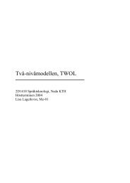
The simulation has been done in a two-dimensional plane (Oyz) of size 2πx2π.
The eddies are generated every dt=0.01s in the center of every 128x128 grid cells
with a spatial step of △y = △z ≈ 0.1σ. In the Fig. 4.1 we can see the plane
surrounded by the eddies generated in the box. In fact this can be seen as passing
a uniform stream through a grid in wind-tunnel experiments.
After defining the discretization, the simulation data has been chosen as following:
• The mean flow: U0 = 10m/s in the x-direction normal to the plane
• The rms velocity: u ′
0 = 1m/s
Using the Reynolds stresses tensor previously defined (Eq. (4.1)) and the turbulent
kinetic energy (Eq. (4.2)), it follows:
⎛
⎜
⎝
1 0 0
0 1 0
0 0 1
which will simplify our problem as expected.
Moreover the parameters to change correspond to :
32
⎞
⎟
⎠ (4.3)

4.1. HOMOGENEOUS ISOTROPIC TURBULENCE (HIT)
Figure 4.1. Inlet plane of eddy generation, surrounded by a box of eddies . 128x128
two-dimensional grid. Simulation of isotropic turbulence with the SEM.Taken from
Ref. [18]
• N ∈ {10, 100, 1000, 10000} the number of eddies in the box
• σ ∈ {0.25, 0.5, 1}: the length scale
• f which will be a tent or a step function
After defining the setup and the variables to modify we will firstly validate
the method by statistics computations in order to continue with a study of the
parameters influence in space and time simulations.
Remarks concerning the simulations run: The values by default when no specified
will be:
• N = 1000
• σ = 0.5
� �
3
• f(x) = 2 (1− | x |), if x < 1
0, otherwise
Moreover the temporal analysis will be realized on the point (x, y) = (π, π) and
the spatial representation will correspond to the last iteration: 1000.
4.1.3 Statistics
As already mentioned we need firstly to check the validity of the method before any
further study regarding neither the algorithm nor the application in a channel flow.
Thus statistics output of simulations, see Fig. 4.2, will be compared to the theory
33

CHAPTER 4. RESULTS
previously presented. As we can observe on the Fig. 4.2a, the time averaged ui
converges almost instantaneously to the correct values, it means: < u >= 10 and
< v >=< w >= 0 , as well as the Reynolds stress tensor on the Fig. 4.2b converging
to the initial one (cf. Eq. (4.3)) after 20s. Finally concerning the skewness (Fig.
4.2c) and the flatness (Fig. 4.2d), the computations show the expected value. The
odd moment (here the skewness) tends to zero as in the Eq. (3.22) and the even
moment, the flatness, is different from zero tending to 3.5 as in the Eq. (3.28).
This last equation reminded as following reveals the strong dependence of this last
moment with respect to the parameters selected, contrary to the skewness.
�
1
Fui = 3 + N 4F 3 VB
f Fε σ3 �
− 3
As we can see, the number of eddies N has a major influence on the signal
flatness. As N goes to infinity the flatness tends towards its Gaussian value of 3.
Therefore it will additionally avoid any influence coming from the eddy size. This
is also true for N near zero, the flatness will grow to infinity independently of the
length scale. Moreover, for a fix N, an increase of the ratio VB
σ3 between the volume
of the box of eddies and the cube of the length scale, can also cause an important
increment of the flatness with respect to the value 3. This would mean that the
box of eddies has been insufficiently filled because of a too large box or a too small
eddies size.
Then an optimized combination of both variables should be studied regarding
the flatness required. However for computational reasons the value of N, which
plays a major role, should be kept as small as possible.
We have to notice that the large fluctuations appearing at the beginning means
that the averaging time is too small. We can compare this fact to the time averaged
sinusoid as in Eq. (4.4)
1
T
� T
sin(wt)dt → O
0
� �
1
T
(4.4)
Once the implementation has been validated we check the influence of the parameters
allowing us to understand better the functioning of the SEM algorithm.
4.1.4 Parameters influence: Spatial and temporal analysis
As expected, the Fig. 4.3 shows how the signal is stationary in time and homogeneous
and isotropic in space. This computation corresponds to a balanced combination
of the parameters with a number of eddies N=1000 and a medium size σ = 0.5
Then in the next simulations just one of the velocity components will be observed.
4.1.4.1 Eddies number(N)
Firstly we will study the effect of the number of eddies on the synthetic velocities
generation. Here three cases will be presented on the Fig. 4.4 for N=10, N=100
34

4.1. HOMOGENEOUS ISOTROPIC TURBULENCE (HIT)
a b
c d
Figure 4.2. Time history of time averaged ui (a), u ′
iu ′
j (b), skweness (c) and flatness
(d)
and N=10000 using a length scale σ = 1. As expected the less eddies are present,
the more are the empty regions without any fluctuation as well in time than in
space domain, whereas higher are the amplitude of the eddies. This is explained
by the concentration of energy on the few eddies. In fact Jarrin [18] proves this
idea through the probability density functions of the velocities which show that the
energy of the signal does not depend on the number of eddies.
Moreover we can clearly observe in the case N = 10 , the travel time of the eddy
through the plane which corresponds to the period of time of the peak, known as
the time scale τ = 2σ
U . However more the number of eddies is increased and more
difficult is to discern these moments because of a higher frequency.
4.1.4.2 Length scale (σ)
Then we investigate the influence of the size of the eddies σ by running some simulations
for values of σ = 0.25, 0.5 and 1 shown on the Fig. 4.5. As expected the
bigger σ is, the larger the length and time scales of the signal are.However if one
reduces the size of the eddies without adding more eddies inside of the box then the
region of influence will be finer causing a higher irregularity and intermittence of
the turbulent signal. Finally as for the previous case, we can observe the time scale
τ = 2σ
U which actually increases for bigger eddy sizes. However when σ is small the
frequency is much higher.
35

CHAPTER 4. RESULTS
Figure 4.3. Spatial representation (left) and time-history of the velocity u, v, w at
point (π, π) (right), for N=1000 and σ = 0.5
36

4.1. HOMOGENEOUS ISOTROPIC TURBULENCE (HIT)
Figure 4.4. Spacial representation (left) and time-history of the velocity u at point
(π, π) (right), for N=10,N=100, N=10000 from top to bottom and σ = 1
37

CHAPTER 4. RESULTS
Figure 4.5. Spacial representation of the velocity w (left) and time-history of v
at point (π, π) (right), for σ = 0.25m, σ = 0.5m, σ = 1m from top to bottom and
N=1000
38

4.1. HOMOGENEOUS ISOTROPIC TURBULENCE (HIT)
4.1.4.3 Distribution function
Finally in the Fig. 4.6 we can have an overview of the influence on the SEM due
to the choice of the distribution function. For that we compare the two following
shape functions:
• A tent function (left)
� �
3
f(x) = 2 (1− | x |), if x < 1
0, otherwise
• A step one(right)
f(x) =
� 1
√2 , if x < 1
0, otherwise
The results observed on the Fig. 4.6 are the consequence of the following fact:
the signal using a step function contains more energy at high frequencies than the
other signal. In fact the energy spectrums shown by Jarrin [18] confirm this point.
Since the shape function defines the eddy, we understand the change of shape,
for the first case spherics and for the second cubic.
Figure 4.6. Influence of the shape functions in the SEM eddies generation. Spacial
representation of the velocity v using a tent function (left) and a step function(right),
for σ = 0.5 and N=1000
After having validated and understood the method for a HIT case it will be
extended to a channel flow computation. Before inserting it into elsA, the previous
code will be extended to a general case namely,a non-HIT, in order to check the
new SEM behaviour and insert it into elsA.
39

4.1.5 Transition to a Non-HIT
CHAPTER 4. RESULTS
In this section the code has been then applied to a general case as a first extension
to a channel case. Now the code takes into account general input data namely the
variation of the mean velocities and a Reynolds stress tensor corresponding to an
inlet plane closed by two parallel walls as shown in Fig. 4.8a and 4.7 respectively .
As we can see in the Fig. 4.7, the autocorrelation terms of the Reynolds stress tensor
reveals the presence of walls by colors (the same phenomenon for the crosscorrelation
terms), showing velocity layers, homogeneous along the walls and with zero value at
the walls (cf. the velocity profiles in Fig. 4.7). (Remark: the orientation of the walls
has been inverted to a vertical position in Fig. 4.7) In Fig. 4.8a we can observe the
same behavior for the mean velocity U and after the SEM computation we obtain
the synthetic velocities with the corresponding profiles of u,v,w as seen in Fig 4.8b.
The homogeneous layers have been then disturbed by the eddies fluctuations and
the new velocity profiles show as well fluctuations along the mean values. Then we
notice clearly the presence of the walls compared to the HIT case with a generated
turbulence along the walls in the streamwise direction x.
The SEM behaving as expected with walls, this code will be applied to a channel
case in the elsA package.
Figure 4.7. Autocorrelation terms of the Reynolds stress tensor
40

4.2. CHANNEL FLOW COMPUTATIONS
a b
Figure 4.8. Input mean velocities (a) and SEM synthetic velocities (b) with their
respective velocity profiles
4.2 Channel Flow Computations
4.2.1 Spatially Developing Channel Flow
4.2.1.1 A Modified SEM
Real reproduction of the non-isotropic nature of the turbulence in the near-wall
region, requires a slight modification of the SEM compared to the previous chapter.
Up to now it was assumed that the length scale σ is the same for all velocity
components and for all directions. However it has been shown that this is not
the case and that streamwise elongated coherent structures dominate the near-wall
region instead of isotropic structures [18]. Thus a different length scale σij is used
for every eddy i of the plane but also for each direction j. Thus we can express:
• The box of eddies B
x j,min = min
x∈S, j∈1,2,3 (xj − σij(x)) and xj,max = max
x∈S, j∈1,2,3 (xj + σij(x))(4.5)
• Velocity signal
ui = Ui + 1
√ N
N�
c k i fσ(x − x k ) (4.6)
k=1
whith the shape function fσ(x − x k ) of the eddies on position i given by
fσij (x − xk) = � VB. 1
σi1
f( x1 − xk 1
).
σi1
1
σi2
41
.f( x2 − xk 2
).
σi2
1
σi3
f( x3 − xk 3
) (4.7)
σi3

4.2.1.2 Implementation
CHAPTER 4. RESULTS
In this section the modified SEM derived from the previous validated code will finally
be integrated in elsA which is a CFD software package for numerical simulation of
turbulent compressible flows.
The implementation has been then split into three parts:
• Python script: for the input parameters and channel configuration
• C++ methods: for the SEM initialization and call of the fortran subroutine
• Fortran subroutine: for the generation of the synthetic velocities per time step
As following the different sections will be discussed more in detail in order to
understand the main roles and the overall functioning and interaction between these
3 sections.
Python elsA
elsA code uses a user interface to describe a computational case, to carry it out and
extract the results from it, in particular for post-processing and analysis. This user
interface uses an Object-Oriented (O-O) conception, like the elsA kernel, but is implemented
in a different O-O language (Python) and uses a simpler set of concepts,
limited to the description of CFD cases. The high level interface provides interface
classes : these interface classes, whose instances are the description objects, completely
define -along with a few functions- the possibilities of user communication
with the kernel, that is the interaction model.
Then the script has been fragmented as following: The main file where the whole
elsA code running is managed, defines firstly the CFD Problem, the model, the Numerics
(in time and space), the viscous flux and imports the other files determining
the boundary conditions, the topology, the parameters and the variables to extract.
In the topology file the domain is divided into blocks linked to a processor. The
type of the boundaries corresponding to the entry face and output face has then
been modified as inlet and outlet respectively. In the parameters file the number
of iteration and the time step can be managed. In the boundary conditions file the
SEM input data N, σ and the Reynolds stress tensor, given through a file name,
has been added. In fact an additional file regarding the Reynolds stress terms has
been generated from another DNS simulation. This has required firstly a symmetry
computation of the values for the other half channel and also an interpolation to
the finer domain of elsA as seen on the Fig. 4.9. Additionally a change of the data
orientation respecting the new rotated axes has been necessary and finally a new
dimensioning has been carried out applying a constant factor.
It is also required the integration of new KEY variables inside the elsA code in
order to be interpreted by the Python scripts and used afterwards by the code in
42

4.2. CHANNEL FLOW COMPUTATIONS
Figure 4.9. Symmetry and interpolation of the input data namely the streamwise
velocity U and the autocorrelation terms of the Reynolds stress tensor
C++ and Fortran. Moreover the variables to extract after each computation have
to be specified in the extract file. In our case the conservative variables and the rms
(root mean square) values have been chosen.
Since the user interface is external to the elsA code, we understand the interest
in specifying the SEM parameters in this part, avoiding a compilation for each test
case and therefore saving time.
Once the input data variables have been integrated, the SEM algorithm has to
be inserted into the whole computation.
C++ file
elsA code has been constructed as a very deep and complex tree of folders of specific
functionalities inside the CFD computation. Since the SEM algorithm works on the
boundary conditions the modifications have mainly affected the files related to it.
All the data initialization computations have been inserted and fragmented into
methods which use the input SEM data sent to them as input parameters. In fact
the interaction between the specified SEM data from the python and this SEM
methods has been managed at another level in the folder tree where the SEM KEY
variables values defined in the python file are extracted and sent to the previous
43

CHAPTER 4. RESULTS
function as parameters. The reading of the SEM file related to the Reynolds stress
tensor terms is also done at this level.
Then, once all the data has been initialized, the main SEM computation should
be called. This part will also be exported at another level and in another language,
Fortran, for time optimization reasons.
Fortran file
In this subroutine, the main Synthetic Eddy Method algorithm appears, namely the
computation of the synthetic velocity which is returned as output value per time
step. Actually this is another difference with respect to the first version since the
loop over the time has been removed. The overall elsA code will manage it when
computing the flow. For every time step it will also call the SEM methods and
subroutines in order to use the new inflow boundary conditions.
An important point regarding the division of the code, concerns the implementation
method of the shared variables. In fact for some cases their value don’t have
to be lost by transmission and the addition of global variables in the .h files and a
dynamic allocation memory have been required.
The following Fig. 4.10 summarizes the main idea, giving an overview of the
general procedure of the whole elsA code and the interaction with the SEM.
4.2.1.3 Setup and Simulation
The computational domain dimensions is of 10πδ×2δ×πδ with a grid of 161×101×
81 cells in the streamwise, wall-normal and spanwise directions, respectively. Here
the dimensionalization is done through δ which represents the half of the channel
high. Periodic boundary conditions are applied in the spanwise directions, whereas
no-slip boundary conditions are imposed at the walls. In streamwise direction inlet
and outlet boundary conditions are set. Fig. 4.11 shows the whole setup of the
simulation. SEM velocities are applied as inflow boundary conditions and at the
outlet, the pressure is specified.
The following computations (Fig. 4.12 and 4.13) correspond to 65000 time steps
thus to three full days of computations or one week of work since the simulations
have to be run manually per 5000 iterations. We can then estimate the time per
iteration equal to 4 seconds.
Concerning the configuration of the channel, the friction Reynolds number
Reτ = 395 and the mean flow Reynolds number Re = 6600 with a WALE (Wall
Adapting Local Eddy-Viscosity) model. Moreover the spatial discretization has
been done with Finite Volume method and an implicit Backward Euler method
44

4.2. CHANNEL FLOW COMPUTATIONS
Figure 4.10. Integration of the Synthetic Eddy Method in elsA
has been used for the time discretization with a time step dt of 0.01s. The SEM
parameters chosen are a tent function for the shape function of the eddies and the
number of eddies has been set to 10,000.
Then in the Fig. 4.12a we observe how the synthetic eddies injected on the inlet
plane result on a physical turbulence along the channel and through the time steps.
In fact this is clearly see on the Fig. 4.12b where in the inlet plane eddy velocities
are set along the wall as initial condition whereas in the outlet plane we observe the
developed turbulent flow.
Fig. 4.13 shows another representation computing the iso-rotational of the velocity
u.
45

a
b
Figure 4.11. Setup of the spatial channel flow using the SEM
CHAPTER 4. RESULTS
Figure 4.12. Spatially Developing Channel Flow Computations. Velocity uz
46

4.2. CHANNEL FLOW COMPUTATIONS
Figure 4.13. Iso-rotational of u in a Spatially Developing Channel Flow Computation.
In order to validate the turbulence generated, an additional simulation has been
run as following for a periodic channel case used as a reference.
4.2.2 Periodic Channel Flow
As shown in Fig. 4.14a, the channel flow simulations have been carried out in a
computational domain of dimensions 2πδ × 2δ × πδ with a grid of 81 × 101 × 81
cells in the streamwise, wall-normal and spanwise directions, respectively. Periodic
boundary conditions are applied in the streamwise and spanwise directions, whereas
no-slip boundary conditions are imposed at the walls (cf. Fig. 4.14a) Which means
that initially a turbulence will be applied in the channel and the flow will be reinjected
iteratively in the streamwise and spanwise direction. A period of time or
number of iterations will be necessary until reaching the convergence of statistics.
The simulations performed concern turbulent plane channel flow after 25000
time steps. At this time we can assume that the stationary step has been reached.
Contrary to the first case, the spatially Developing Channel Flow, the channel can
be reduced since the turbulence is developed in time and no in space anymore. Concerning
the configuration of the channel, the same as for the Spatially Developing
Channel Flow has been used and some simulations have been run.
In Fig. 4.14 we can actually observe the turbulent flow channel through different
representations: the velocity w in the streamwise direction (Fig. 4.14b), presented
on the Fig. 4.14c and d by colour on the boundaries and as iso-surfaces, respectively.
We consider that after this period of time, the process is stationary.
47

a b
c d
CHAPTER 4. RESULTS
Figure 4.14. Periodic LES turbulent channel flow. Setup of the domain (a). Representation
of the velocity uz (b). Magnitude of vorticity on boundaries (c) and as
iso-surfaces (d)
4.2.3 Statistics
In this section the first analysis of time averaged statistics extracted from the previous
simulations are exposed. This first step of statistics study will determine the
next steps to achieve as a future work.
Fig. 4.15 and 4.16 give a first overview of the rms (root mean square) of the
streamwise velocity for the periodic and spatial case. These velocities profiles confirm
the previous result in spatial domain where the periodic channel shows to have
reached a stationary state contrary to the spatial one. In fact the periodic case
could be seen as an equivalent infinite channel. However in the spatial channel an
important increase of the fluctuations are shown after 5000 iterations. If we then
compute the flow-through times as following:
n = τNU
L
(4.8)
with the dimensionless values: τ = 0.01, U = 1, L = 10π, N = 60000, we find a
number of times around 20 which could explain a non reached stationary state.
48

4.2. CHANNEL FLOW COMPUTATIONS
Therefore we can also notice on the previous simulations how the turbulence
in the middle of the channel seems to be more developed for the periodic LES
computations than for the spatial channel.
These observations would require an increase of the iterations but also of the
channel size. In order to check if the channel size is enough large, data extraction
should be taken at two different points far in the downstream channel. Similar
results extracted at these two points would validate the selected size.
However a loss of symmetry is observed contrary to the periodic case, which
should be treated.
Finally, contrary to the HIT and as expected, we observe for both cases a zero
velocity on the walls.
Thus these remarks show the need of a further study based on the channel size,
an increase of the time steps number and on SEM parameter variations.
Figure 4.15. Periodic channel statistics for 25000 time steps
49

a b
CHAPTER 4. RESULTS
Figure 4.16. Spatial channel statistics. For 60000 time steps (a) and 65000 time
steps (b)
50

Chapter 5
Discussion
In this project the Synthetic Eddy Method of generating inflow data for LES has
been implemented in the elsA code. The method, based on the classical view of
turbulence as a superposition of eddies has firstly been used in a HIT. The study of
statistics has allowed to validate the method and the variation of the parameters has
revealed the sensitivity of the procedure with respect to them, namely the number
of eddies N, the length scale σ, the distribution function f. However the choice of
these variables should not be taken independently from each other since the results
obtained from every parameter value determined will depend on the configuration
of the others. For example if we want to decrease the eddy size without loosing
an homogeneous spatial distribution of the fluctuations, the number of eddies will
have to be increase. However if we choose a big length scale σ with respect to the
dimension of the plane, the fluctuating signal will be smoother and this time the
number of eddies won’t have any effect. This relation appears clearly through the
influence on the flatness Eq. (3.28).
Then an extension has been possible to a more general and practical case, a
channel flow computation. The simulation has also been run with a periodic LES
as a reference of comparison for the SEM.
Even if physical turbulence have been observed, the periodic case shows higher
turbulence which will require some improvements of the spatially developing channel
flow case. Actually a further study can be done regarding the choice of the parameters,
the size of the channel. Concerning the parameters, the eddy size should be
limited by a fraction of the wall-normal dimension and the number of eddies N as
well as the channel dimensions by a computational cost. Statistics analysis already
started will allow the validation with respect to the periodic LES reference.
Hence the Synthetic Eddy Method has shown to have several advantages as the
elimination of a previous precursor simulation, its application to general flows and
the control of the method by divers parameters defining the eddies. However this
method is mainly based on random variables taking into account just the Reynolds
stress tensor as physical contribution.
Therefore as a future work, even if the SEM has already been tested and vali-
51

CHAPTER 5. DISCUSSION
dated in a wide variety of turbulent flows, further improvements of the algorithm
could eventually been study as for instance the use of the shape function. Moreover
comparisons with spectral methods could be carried out and a coupling with the
RANS domain should be afterwards implemented.
52

Bibliography
[1] J-L. Aider and A. Danet. Large-eddy simulation study of upstream boundary
conditions influence upon a backward-facing step flow. Comptes Rendus
Mecanique, 2006.
[2] Jean-Bernard CAZALBOU. Physique et modélisation de la turbulence,
Théories de la Turbulence Homogène. ISAE, ENSICA, 2008.
[3] C.Hirsch. Numerical computational of internal and external Flows: Fundamentals
of numerical discretisation, vol 1. John Willey & Sons, 1988.
[4] L. Davidson. Using isotropic synthetic fluctuations as inlet boundary conditions
for unsteady simulations. Advances and Applications in Fluid Mechanics, 2007.
[5] J.W. Deardorff. A numerical study of three-dimensional turbulent channel flow
at large Reynolds numbers. Journal of Fluid Mechanics, 1970.
[6] Julien Delbove. Approche des problèmes instationnaires d’interaction fluide/structure
avec elsA. Mémoire de DEA, INP, ENSEEIHT, 2001.
[7] F. Ducros and F. Nicoud. Subgrid-Scale Stress Modelling Based on the Square
of the Velocity Gradient Tensor. Flow, Turbulence and Combustion, vol. 62,
1999.
[8] Manuel Théorique elsA. Spécification Technique de besoins. 2000.
[9] A. Ferrante and S.E. Elghobashi. A robust method for generating inflow conditions
for direct simulation of spatially developing turbulent boundary layers.
Journal of Computational Physics, 2004.
[10] F.Laporte. Simulation numérique appliquée à la caractérisation et aux instabilités
des tourbillons de sillage d’avions de transport. PhD thesis, Institut
National Polytechnique de Toulouse, Spécialité dynamique des fluides, 2002.
[11] R. Friedrich and M. Arnal. Analysing turbulent backward-facing step flow with
the lowpass-filtered Navier-Stokes equation. Journal of Wind Engineering and
its Applications, 1990.
53

BIBLIOGRAPHY
[12] Ulka Gaitonde. Quality Criteria for Large Eddy Simulation. School of MACE,
University of Manchester, 2008.
[13] M.Emmanuel Germaine. Modélisation de la couche limite turbulente instationnaire
pour les simulations aux grandes échelles: Construction et mise en
oeuvre d’une approche "Lois de Parois" dans le logiciel elsA". Master recherchesupaéro,
spécialité: Dynamique des Fluides, Énergétique et Transfert, 2007.
[14] P. Moin H. Le and J. Kim. Direct numerical simulation of turbulent flow over
backward-facing step. Journal of Fluid Mechanics, 1997.
[15] R. Mittal T.S. Lund H.J Kaltenbach, M. Fatica and P. Moin. Study of flow
in a planar asymmetric diffuser using large eddy simulation. Journal of Fluid
Mechanics, 1999.
[16] P. Moin J. Kim and R. Moser. Turbulence statistics in fully developed channel
flow at low Reynolds number. Journal of Fluid Mechanics, 1987.
[17] Nicolas Jarrin. Industrial Use of Large-Eddy Simulation:Numeric, Inlet Boundary
Conditions, Wall Flows and Hanging-Nodes. Department of Mechanical
Aerospace and Manufacturing Engineering, 2004.
[18] Nicolas Jarrin. Synthetic Inflow Boundary Conditions for the Numerical Simulation
of Turbulence. PhD Thesis,faculty of engineering and physical sciences.
University of Manchester, 2008.
[19] R.H. Kraichnan. Diffusion by a random velocity field. Physics of Fluids, 1969.
[20] E. Labourasse and P. Sagaut. Reconstruction of turbulent fluctuations using a
hybrid RANS/LES approach. Journal of computational physics, 2002.
[21] M. Lazareff. elsA , User’s Reference Manual. ONERA, 2007.
[22] M. Lazareff. elsA, Theoretical Manual. ONERA, 2008.
[23] D.K. Lilly. A Proposed Modification of the Germano Subgrid-Scale Closure
Method. Phys. Fluids, vol. A4(3), 1992.
[24] J.L. Lumley. Stochastic tools in turbulence. Academic Press, New-York and
London, 1970.
[25] A. Sadiki M. Klein and J. Janicka. A digital filter based generation of inflow
data for spatially developing direct numerical or large-eddy simulations. Journal
of Computational Physics, 2003.
[26] Pierre Comte Marcel Lesieur, Olivier Métais. Large-eddy simulations of turbulence.
Cambridge University Press, 2005.
54

BIBLIOGRAPHY
[27] Eric Garnier Sébastien Deck Pierre Sagaut Mathieu Pamiès, Pierre-Élie Weiss.
Generation of synthetic turbulent inflow data for large eddy simulation of
spatially evolving wall-bounded flows. Department of Applied Aerodynamic,
ONERA- Institut Jean le Rond d’Alembert, Université Pierre et Marie Curie
France- PHYSICS OF FLUIDS 21, 1, 2009.
[28] D. Laurence N. Jarrin, S. Benhamadouche and R. Prosser. A Synthetic-Eddy-
Method for Generating Inflow Conditions for Large-Eddy Simulations. School
of Mechanical, Aerospace and Civil Engineering (University of Manchester) -
Département Mécanique des Fluides et Transferts Thermiques(Electricité de
France), 2005.
[29] D. Laurence R. Prosser N. Jarrin, S. Benhamadouche. A Synthetic Eddy Method
for generating inflow conditions for LES. University of Manchester, EDF.
[30] R. Prosser D. Laurence N. Jarrin, J-C. Uribe. Synthetic inflow boundary conditions
for wall bounded flows. 2 nd Symposium on Hybrid RANS-LES Methods,
Corfu, Greece.
[31] Y. Addad D. Laurence N. Jarrin, S. Benhamadouche. Synthetic turbulent inflow
conditions for large eddy simulation. Proceedings, 4th International Turbulence,
Heat and Mass Transfer Conference, Antalya, Turkey, 2003.
[32] E. Balaras N. Li and U. Piomelli. Inflow conditions for large-eddy simulation
of mixing layers. Physics of Fluids, 2000.
[33] Uribe Uribe A. RevellRevell R. Prosser D. Laurence Laurence N.Jarrin Jarrin,
J. LES fines et méthodes hybrides RANS/LES. University of Manchester, EDF,
DESider, 2007.
[34] E. Tromeur L. Larcheveque P. Sagaut, E. Garnier and E. Labourasse. Turbulent
inflow conditions for LES of compressible wall bounded flows. AIAA Journal,
42(3), 2004.
[35] M. Strelets P. Spalart and A. Travin. Direct numerical simulation of large-eddy
breakup devices in a boundary layer. International Journal of Heat and Fluid
Flow, 2006.
[36] Jean philippe Boin. Turbulence. ENSIB, 2001-2002.
[37] Ugo Piomelli. Wall-layer models for large-eddy simulations. Elsevier. Progress
in Aerospace Sciences 44, Department of Mechanical and Materials Engineering,
Queen’s University, Kingston, Ontario, Canada K7L 3N6, 2008.
[38] S. Pope. Turbulent flows. Cambridge University Press, 2000.
[39] M.M. Rai and P. Moin. Direct numerical simulation of transition and turbulence
in a spatially evolving boundary layer. Journal of Computational Physics, 1993.
55

BIBLIOGRAPHY
[40] R.S. Rogallo. Numerical experiments in homogeneous turbulence. Nasa TM-
81315, 1981.
[41] T.P. Parr D.M. Hanson-Parr R.R. Grinstein, E.J. Gutmark and U. Obeysekare.
Streamwise and spanwise vortex interaction in an axysymmetric jet. a computational
and experimental study. Physics of Fluids, 1996.
[42] S.K. Lele S. Lee and P. Moin. Simulation of spatially evolving turbulence and
the applicability of Taylor’s hypothesis in compressible flow. Physics of Fluids
A, 1992.
[43] J. Smagorinsky. General circulation experiments with the primitive equations:
I The basic equations. Monthly Weather Review, 1963.
[44] Nicolas Jarrin Sofiane Benhamadouche and Dominique Laurence Yacine Addad.
Synthetic turbulent inflow conditions based on a vortex method for
large-eddy simulation. Progress in Computational Fluid Dynamics, Vol. 6,
Nos. 1/2/3,EDF R&D Dept. MFTT,UMIST,MAME Dept. Thermo-Fluids div.,
2006.
[45] X. Wu T. Lund and D. Squires. Generation of turbulent inflow data for
spatially-developing boundary layer simulations. Journal of Computational
Physics, 1998.
[46] M. Wang and P. Moin. Computation of trailing-edge flow and noise using
large-eddy simulation. AIAA Journal, 2000.
[47] Jean-Philippe Boin Yann Colin. Technical notes: Driving state definition and
normalization within elsA-Python script. 2006.
56

TRITA-CSC-E 2009:112
ISRN-KTH/CSC/E--09/112--SE
ISSN-1653-5715
www.kth.se