Systematically Misclassified Binary Dependant Variables

School of Economic Sciences 

Working Paper Series 

WP 2011-9 

Systematically Misclassified Binary 

Dependant Variables 

By 

Vidhura Tennekoon and Robert Rosenman 

July 2011

SYSTEMATICALLY MISCLASSIFIED BINARY DEPENDANT VARIABLES 


VIDHURA TENNEKOON a AND ROBERT ROSENMAN b 

JULY, 2011 

a Graduate Student, School of Economic Sciences, Washington State University, Pullman, WA 

99164, USA. vidhura@wsu.edu. 1-509-335-5556. Fax 1-509-335-1173. Corresponding author. 

b Professor, School of Economic Sciences, Washington State University, Pullman, WA 99164, USA. 

yamaka@wsu.edu. 1-509-335-1193. Fax 1-509-335-1173. 

1



SUMMARY 

When a binary dependant variable is misclassified probit and logit estimates are biased 

and inconsistent. In this paper we suggest a conceptual basis for endogenous 

misclassification of the dependant variable due to systematic respondent bias and the use 

of Likert scales commonly used in measuring categorical variables. We develop an 

estimation approach that corrects for endogenous misclassification, validate our 

approach using a simulation study and apply it to the analysis of a treatment program 

designed to improve family dynamics. Our results show that endogenous misclassification 

could lead towards potentially incorrect conclusions unless corrected using an 

appropriate technique. 

Key words: misclassification, response shift bias, Likert scale, treatment evaluation 

JEL codes: C21,C31,C51,I10,I12. 

2


1. INTRODUCTION 1 

Misclassification of a categorical variable occurs when an observation is listed in a 

category than where it truly belongs. If the outcome variable can take on values in J 

mutually exclusive categories, the “true” value can be incorrectly classified into one of the 

remaining J-1 categories, resulting in J ( J −1) 

ways that the outcome could be 

misclassified. In the dichotomous case misclassification means that one or more of the 

observations in the outcome variable with a true value of ‘0’ are observed as ‘1’, or one or 

more of the true ‘1’s are observed as ‘0’s, or both. When the misclassified variable 

happens to be the dependant variable, probit or logit estimates may lead to biased and 

inconsistent estimates if the misclassification is ignored or modeled incorrectly (Hausman, 

2001). 

Misclassification of a variable can happen for various reasons, although one can 

categorize them broadly into two reasons; response error on the part of the individual 

being observed, or data (entry) error which occurs after a respondent has given a 

response. In labor market data, for example, some respondents may misreport their 

employment status or a correctly reported labor status may be mistranscribed (Chua and 

Fuller, 1987 ; Poterba and Summers, 1995). If the misclassification is due to response 

error, the error is often unambiguous. In the labor market case, for example, there 

should be no obstacle to unambiguously observing one’s own employment status, and in 

1 This research was supported in part by a grant from the National Institute of Drug Abuse (R21-DA 025139- 

01Al). We thank the parents and facilitators who participated in the program evaluation of SFP. We also 

thank Ron Mittlehammer, Laura G. Hill, Dan Friesner and Sean Murphy for many useful comments and 

Jason Abrevaya for sharing his Gauss code used for estimating the model presented in Hausman et al. 

(1998). 

3


any case an outside observer should be able to correctly identify the response error given 

the same information as the respondent. Moreover, a properly informed respondent 

who understands the question and categories would have no problem assigning herself 

correctly. 

However, not all response errors are so unambiguously identified. For example, 

when a medical condition has no clear objective measure, patients’ perceptions of 

improvement are subjective (Murphy et al., 2011). Self-reported measures of an outcome 

are most commonly used when no objective measure exists. Such a case is more 

complicated than when there are objective measures because a respondent may 

misreport her category genuinely believing that it is correct, and the misclassification is 

thus integrated into the measurement process. If such misreporting is systematically 

related to covariates of the respondents true category, then misclassification is 

endogenous to the model. This is the case we explore here, when the probability of 

misclassification is observation specific and dependent on covariates, and there is no 

objective measure of which category is correct. 

Subjective measurement, of course, need not lead to misclassification. In a 

conceptual sense, it may seem impossible for a subjective measure to be “wrong”. 

However, most empirical analysis requires some sense of comparison of measures across 

individuals. We see two potential sources for endogenous misclassification. The first is a 

systematic bias, compared to others offering their own assessments, that depends on 

covariates that may or may not also determine the assessment. For example, in “before” 

4


and “after” studies of a treatment, the anchoring of responses to the first measure can 

lead to systematic bias in the second. Program evaluators and quality of life researchers 

often refer to such a case as “response shift” bias (Schwartz and Sprangers, 1999; 

Brossart et al., 2002). Murphy, et. al. (2011) show a framing effect that also can lead to a 

systematic bias that differs from a response shift bias. 

A second potential source of misclassification comes from the measurement 

instrument itself. When assignment is subjective, it is usual to offer several categories of 

subjective evaluation using a Likert-type scale. For example, in medical studies, the 

categories of choice after a treatment might include several gradations from “made much 

better” to “made much worse.” Such a measuring stick can also lead to misclassification 

due to what we term “Likert imbalance bias”. 2 

Previous work on misclassified dependant variable includes Chua and Fuller 

(1987), Poterba and Summers (1995), Hausman et al. (1998), Abrevaya and Hausman 

(1999), Lewbel (2000) and Dustmann and van Soest (2000). Chua and Fuller (1987) 

present a useful parametric model that can be estimated using Non-Linear Least Squares, 

incorporating all J ( J − 1) misclassification possibilities of an outcome variable with J 

categories. The procedure, however, requires a minimum of three independent sets of 

survey responses by re-interviewing the original respondents, and has a limited practical 

usage. The conditional logit procedure proposed in Poterba and Summers (1995) also 

incorporates all possibilities of misclassification and requires misclassification 

2 In the appendix we expand on this idea. 

5


probabilities found by analyzing the discrepancies between interview and re-interview 

outcomes. 

Hausman et al. (1998) and Abrevaya and Hausman (1999) extend the analysis 

when misclassification probabilities cannot be independently verified to provide 

parametric estimators of a model when the functional form of the distribution of the 

error term is known. The focus of Hausman et al. (1998) is a dichotomous outcome 

variable with two types of misclassification, which they denote as α 

0 

(the probability that 

a true 0 is recorded as a 1) and α 

1 

(the probability that a true 1 being recorded as 0) 3 . 

They also provide a semi-parametric estimator for the case where the distribution of the 

error is unknown and the misclassification probabilities are constant (independent of all 

covariates). With their parametric approach the unknown misclassification probabilities 

are estimated simultaneously with the usual coefficients of the binary choice model. Their 

semi-parametric method provides consistent estimates of the model parameters, but not 

of the misclassification probabilities. 

In Lewbel (2000), the misclassification probabilities α 

0 

and α1 

are allowed to be 

covariate-dependant functions. The author shows that (given some regularity) the binary 

choice model with covariate-dependant misclassification is completely identified even 

when the functions α 

0 

, α1 

and the distribution of the error term are unknown. However, 

as the author acknowledges, his estimators are ‘not likely to be very practical since they 

involve up to third order derivatives and repeated applications of nonparametric 

3 Throughout this paper we use the same notation. 

6


regression’ (pp. 607-608 ). Non-availability of any empirical work exploiting the 

estimators proposed in Lewbel (2000) so far indicates the importance of a more practical 

estimator, even at the cost of some functional form assumptions. 

Dustmann and van Soest (2000) extend the parametric model of Hausman et al. 

(1998) to a trichotomous case and apply it to analyze the speaking fluency of male 

immigrants in Germany. Their application, which uses self-reported data, is more related 

to the case discussed here than most early research on the subject, which focuses on 

labor market outcomes. However, Dustmann and van Soest (2000) maintain the 

assumption that all misclassification probabilities are constants. 

Our paper extends the parametric approach of Hausman et al. (1998) in a different 

direction, generalizing their estimator to the case, where the misclassification 

probabilities are not constants, but instead are functions of one or more covariates 4 . The 

parametric estimator that we propose here is a more tractable way to identify the same 

model as Lewbel (2000), conditional on functional form assumptions. The paper proceeds 

as follows. In section 2, we present our structural approach to deal with covariantdependant 

misclassification of the dependent variable and the identification 

requirements. Section 3 has a Monte Carlo experiment that compares our model with 

the ordinary probit model and the basic model presented in Hausman et al. (1998). In 

section 4, we present an empirical application to demonstrate the applicability of the 

4 Although such an extension is briefly discussed in section 5.5 of HAS, they do not fully characterize or 

implement the approach. A semi-parametric approach to deal with covariate-dependent misclassification of 

the dependent variable is discussed in detail in Abrevaya and Hausman (1999). Our interest, however, is in 

the parametric model. 

7


model. Finally, in section 5 we discuss implications and conclusions from our 

generalization. 

2. THE GENERALIZED MODEL TO CORRECT FOR COVARIATE-DEPENDANT 

MISCLASSIFICATION 

Assume, 

* 

yi 

is an unobserved latent variable such that 

y = X β + ε 

(1) 

* 

i i i 

where, 

X 

i 

is a vector of observed independent variables, β is a vector of coefficients to 

be estimated and εi 

is an iid error term with a known common distribution. We observe 

y 

i 

= ≥ (2) 

* 

1( yi 

0). 

If no misclassification is present, we always observe the dichotomous outcome variable, 

y 

i 

, correctly. However, if there is misclassification the outcome variable that we observe, 

o 

y 

i 

, includes some true ‘1’s classified as ‘0’s and some true ‘0’s classified as ‘1’s. As a 

result, in general, 

y 

o 

i 

≠ 

y . Following Hausman et al. (1998), we denote the constant 

i 

misclassification probabilities as follows: 

o 

( yi 

yi 

) 

α 

0 

= Pr = 1| = 0 

(3) 

o 

( yi 

yi 

) 

α 

1 

= Pr = 0 | = 1 

(4) 

It follows that the overall stochastic mechanism that determines the values ultimately 

observed with random misclassification is a conditional Bernoulli process that can be 

characterized via the following general data generating process: 

8


y = 1( y ≥ 0)1( u ≤ 1 − α ) + 1( y < 0)1( u ≤ α ), where u ~ Uniform 0,1 , 

∀ i 

(5) 

0 * * 

i i i 1 i i 0 

i 

( ) 

and ε 

i 

in (1) and u 

i 

are independent. If the values of α0 

and α1 

are dependent on y i 

as in 

(3) and (4), but independent of X 

i 

, and the probability distribution function of εi 

is F (.) 

then, as Hausman, et al. show, we can express the expected value of the observed 

dependant variable as 

o 

o 

( ) ( ) 

( ) 

E y | X = Pr y = 1| X = α + 1 −α − α F( X β ) 

i i i i 0 0 1 

i 

(6) 

When α0 

and α1 

are constants and α0 + α1 < 1, 5 the parameters of the above model can 

be consistently estimated either by MLE or NLLS 6 . 

Suppose instead that the misclassification probabilities α0 

and α 

1 

are functions of 

a set of variables, 

0 

Zi 

and 

1 

Z i 

respectively as in Lewbel (2000). In particular, the 

probabilities in (3) and (4) are now given by 

α 

( ) ( 

Z = Pr y = 1| y = 0, 

Z = 

F Z 

γ 

0 o 

0 0 

0 i i i i 0 i 

0 

( ) ( 

) ( ) 

) ( ) 

α 

Z = Pr y = 0 | y = 1, 

Z = 

F Z 

γ 

1 o 

1 1 

1 i i i i 1 i 

1 

(7) 

(8) 

where 

0 

Zi 

and 

1 

Zi 

are subsets 7 of X 

i 

and F 

0 

and F1 

are the cumulative distribution 

functions of stochastic components that determine each type of misclassification 8 . 

5 This condition, termed as the monotonocity condition in Hausman et al. (1998) must be satisfied to 

( β, α , α ) 

( −β,1 −α ,1 − α ) . 

identify 

0 1 

separately from 

1 0 

6 The relevant objective functions are given by equations (6) and (7) in Hausman et al. (1998). 

7 This also includes the case that one or both misclassification probabilities depend on variables that do not 

affect the true outcome since X 

i 

may include variables with coefficients equal to zero. 

8 Of course, one could elaborate on this specification and provide a latent variable structure to the 

underlying misclassification probabilities that would lead to the CDF specification in (6) and (7). A 

9


Inserting the preceding generalized representation of the misclassification probabilities 

into (6), the expected value of the observed dependant variable with a covariatedependant 

misclassification can be defined as: 

( ) 

o 0 1 o 

0 1 0 0 1 

( ) ( ) 0 ( 0 ) 0 ( 0 ) 1 ( 1 ) 

E y | X , Z , Z = Pr y = 1| X , Z , Z = F Z γ + 1 − F Z γ − F Z γ F( X β ) (9) 

i i i i i i i i i i i i 

If the first elements of vectors 

0 

Zi 

and 

1 

Zi 

are constants and the vectors 

γ 

i 

= 

⎢ 

⎡γi0 

⎤ 

⎢ 

. 

⎥ 

⎢ ⎥ 

⎢ . ⎥ 

⎥ 

⎢ . ⎥ 

⎢ 

⎣γ 

⎥ 

in ⎦ 

for 

i = 0,1 with γij 

≠ 0 for j = 0 and γ 

ij 

= 0 for j > 0 we have α 

i 

= F( γ 

i0) 

in (5). 

Accordingly, equation (9) nests the basic model (model 1) presented in Hausman et al. 

(1998), which is a statistically testable proposition. 9 

Assuming the functional forms of F0 , F 

1 

and F are known the parameters of the 

model can be estimated with NLLS by minimizing 

( ( ) ) 2 

i i i i i 

n 

( ) 0 ( 0 ) ( 0 ) ( 1 

0 1 

= − 

0 0 

− − 

0 0 

− 

1 1 ) 

f β , γ , γ ∑ y F Z γ 1 F Z γ F Z γ F( X β ) 

(10) 

i= 

1 

over( β, γ , γ ) . Alternatively, MLE can be applied to the following log likelihood function: 

l 

( β, γ , γ ) 

0 1 

0 1 

= n 

−1 

( ) 

( ) 

0 0 0 1 

y ⎡F0 ( Z 

0 ) F0 ( Z 

0 ) F1 ( Z 

1) 

F X 

⎣ 

0 0 0 1 

( ) ⎡ 

0 ( 0 ) 0 ( 0 ) 1 ( 1) 

⎛ 

n i 

ln 

i 

γ + 1 − 

i 

γ − 

iγ ( 

iβ) 

⎤ + ⎞ 

⎜ 

⎦ ⎟ 

∑ (11) 

i= 

1 ⎜ 1− yi ln 1− F Zi γ − 1 − F Zi γ − F Ziγ F( Xiβ 

) ⎤ ⎟ 

⎝ ⎣ 

⎦ ⎠ 

generalization of the model could include a correlated error structure between the error terms of the latent 

variable equations. 

0 1 

F Z = F Z ≡ (9) further collapses to a standard binary choice specification. 

9 Moreover, if ( i 

γ ) ( i 

γ ) 

0 0 1 1 

0, 

However, as discussed in footnote 10, it is not possible to directly test for this. 

10


In the Monte-Carlo simulations and the application to real data that we present in 

subsequent sections, all the parameter estimations are based on MLE using equation (11). 

We also assume that all three error terms are distributed normally. 

As we explained earlier, HAS1 is a special case of our generalization, which we 

refer to hereafter as GHAS, without any covariates affecting each type of misclassification 

probabilities. The generalization of the Hausman et al. (1998) data generating process in 

(5) that applies to the GHAS specification is given by: 

( ) 

( ) ( ) 

y = 1( y ≥ 0)1( u ≤1 − F Z γ ) + 1( y < 0)1( u ≤ F Z γ ), 

0 * 1 * 0 

i i i 1 i 1 i i 0 i 0 

where u ~ Uniform 0,1 , ∀ i 

i 

(12) 

and again ε 

i 

in (1) and u 

i 

are independent. The nesting of HAS1 in GHAS and of the 

standard binary choice model in HAS1 facilitates statistical testing for the most suitable 

model in a given application. The significance tests for parameters in 

0 

Zi 

and 

1 

Z 

i 

other 

than the constant terms serve as tests for the suitability of GHAS over HAS1. Given that 

no other elements of 

0 

Zi 

and 

1 

Z 

i 

pass this threshold, one may estimate HAS1 and the 

significant tests of the terms α0 

and α 

1 

serve as tests for the suitability of HAS1 model 

over the standard binary choice model 10 . 

10 The standard probit model is not nested in GHAS in a directly testable manner and thus we propose this 

sequential procedure. As the misclassification probability, 

αk 

for k = 0,1reaches 0, 

Z γ approaches the 

lower bound of F (.) 

which is −∞ in case of a normal distribution, potentially leading to convergence 

issues. As such, convergence issues of GHAS may indicate a misspecified model. 

k 

i 

k 

11


Identification of the parameters of (11) stems from the non-linearity of F0 , F 

1 

and 

F . The first order necessary conditions and the Fisher information matrix of (11) can be 

expressed as below. 

⎡ ∂L 

⎤ 

⎢ ⎥ 

⎢ ∂β 

⎥ 

n 0 

0 

⎢ ∂L 

⎥ ⎛ 

−1 

y ( 1− 

yi 

) ⎞ 

g = n 

i 

⎢ ⎥ = ∑ 

− C 

0 

1 

( 1 ) 

i 

= 0 

∂γ 

⎜ P 

i= 

i 

− P ⎟ 

⎢ ⎥ ⎝ i ⎠ 

⎢ ∂L 

⎥ 

⎢ ⎥ 

⎣ ∂γ 

1 ⎦ 

(13) 

2 2 2 

⎡ ∂ L ∂ L ∂ 

L 

⎤ 

⎢ 

⎥ 

∂β ∂β ∂β ∂γ ∂β ∂γ 

' ' ' 

⎢ 

0 1 ⎥ 

⎢ 2 2 2 

n 

∂ L ∂ L ∂ 

L 

⎥ ⎛ ⎞ 

−1 1 

' 

⎢ 

' ' ' 

⎥ ∑ 

i i 

∂β ∂γ 0 

∂γ 0∂γ 0 

∂γ 0∂γ 

⎜ 

1 

i= 

1 P ⎟ 

i i 

I = − E = n C C 

⎢ ⎥ ⎝ ( 1− 

P ) ⎠ 

⎢ 2 2 2 

∂ ∂ ∂ 

⎥ 

⎢ 

L L L 

⎥ 

' ' ' 

⎢⎣ 

∂β ∂γ 1 

∂γ 0∂γ 1 

∂γ 1∂γ 

1 ⎥⎦ 

( ) 

0 0 1 

where 

0 ( 0 ) 0 ( 0 ) 1 ( 1) 

P = F Z γ + 1 − F Z γ − F Z γ F( X β ) , 

i i i i i 

(14) 

( − 

0 ( 0 ) − 

1 ( 1) 

) 

⎡ 

⎢ 

C = ⎢ 1 − F( X ) F ( Z γ ) Z 

0 1 ' 

1 F Zi γ F Zi γ F ( X 

iβ 

) X 

i 

( β ) 

' 0 0 

i i 0 i 0 i 

⎢ 

' 1 1 

−F( X 

iβ 

) F1 ( Zi γ1) 

Zi 

⎢ 

⎣ 

⎤ 

⎥ 

⎥ and 

⎥ 

⎥ 

⎦ 

F , F and 

' 

0 

' 

1 

' 

F are the first derivatives of 

F0 , F 

1 

and F respectively. 

When F 

0 

and F are symmetric and F1 = F0 

identification requires that 

different from 

1 

Z 

i 

. To demonstrate that consider the case where 

0 

Z 

i 

be 

Z = Z = Z , F ( v) = F ( v) = 1 − F ( −v) 

and F( v) = 1 − F( − v) 

. Then the log-likelihoods, 

0 1 

i i i 

1 0 0 

12


l 

l 

( β , γ , γ ) = ( −β , −γ , − γ ) . Hence, to identify ( , , ) 

0 1 1 0 

β γ γ from( −β, −γ , − γ ) , we 

0 1 

1 0 

need Z 

0 ≠ Z 

1 . A merit of our estimator, however, is that the identification does not 

i 

i 

0 

1 

0 1 

require X ≠ Z or X ≠ Z when Z ≠ Z and F (.) , 0 

F (.) 1 

and F (.) are non-linear 

i 

i 

i 

i 

i 

i 

transformations. Additional exclusive restrictions will certainly help strong identification 

0 1 

of parameters but are not necessary. Moreover, if Z ≠ Z we no longer need α0 + α1 < 0 

as Hausman et al. (1998) requires. In spite of these advantages our estimator has certain 

limitations too. The Hausman et al. estimator allows the misclassification probabilities to 

be zero (but not 1, since that would violate the monotonicity condition). Ours require 

each type of misclassification probabilities to be bounded between 0 and 1, and not at 

the possible extremes, because if either of the two types of misclassifications takes an 

' 

extreme value, the matrix C C becomes singular. A related consequence would be very 

i 

i 

large standard errors when misclassification probabilities are too small or too large. In 

contrast to HAS1, our estimator performs best when the misclassification probabilities 

are large in both directions 11 . 

3. MONTE CARLO EXPERIMENT 

We set up a Monte Carlo experiment which mimics the experimental setup in 

Hausman et al. (1998) in order to assess the impact of covariate-dependant 

misclassification on estimates with and without an appropriate correction mechanism. 

We first generated the X matrix in equation (1) including three random variables and a 

i 

i 

11 If the misclassification is one-sided we can use a restricted version of our model, circumventing this 

identification issue while improving the efficiency of the estimator. 

13


constant as covariates. Our X matrix is identical to the one they use in section 4 of their 

paper and comprises of x 

1 

, drawn from a lognormal distribution, x 

2 

, a dummy variable 

equal to one with probability 1/3, x 

3 

, a random variable distributed uniformly, and a 

constant. The econometric error term, ε , was drawn from a standard normal 

distribution. The parameter vector β also is identical to theirs. Based on this data 

generation process, the latent dependent variable is given by, 

= + where X = [ 1 x x x ], [ ] 

* 

y X β ε 

1 2 3 

β = − 1 0.2 1.5 0.6 ' 

(15) 

However, in our experiment the two types of misclassification probabilities are 

not constants; instead they are functions of subsets of X . More specifically, we have 

designed our experiment such that, the covariates in equations (6) and (7) are given by 

Z 

= [ 1 x ] and Z [ 1 x x ] 

0 3 

= . 

1 2 3 

If we denote γ = [ γ γ ] and γ [ γ γ γ ] 

0 00 01 

= , given the distribution of Z 

0 

1 10 11 12 

and Z 1 

, we can define the expected values of α0 

and α 

1 

in equations (8) and (9) 

respectively as, 

γ + γ 

00 01 

( 0 ) = ⎡Φ ( 0 0 ) ⎤ = Φ ( ) 

E α E ⎣ Z γ ⎦ ∫ θ dθ 

(16) 

γ 

00 

γ + γ + γ γ + γ 

10 11 12 10 12 

( α1 ) = ⎡ ( 1γ 1) 1 ( θ ) θ 2 

⎣Φ ⎤⎦ = ∫ Φ + ∫ Φ ( θ ) θ 

(17) 

E E Z d d 

3 3 

γ γ γ 

10 + 11 10 

where Φ( θ ) denotes the normal distribution function. For consistency with the 

Hausman et al. (1998) experiment, we choose the parameter vectors γ 

0 

and γ 

1 

such that 

the expected value of each of the two types of misclassification probabilities are both 

14


approximately equal to our desired values for α0 

and α 

1 

(0.02, 0.05, 0.1 or 0.2), by 

numerically integrating (16) and (17) using Gauss-Legendre quadrature. We also ran two 

more sets of Monte Carlo runs with asymmetric misclassification for ( α0, α 

1) 

=(0.02, 0.2) 

and (0.2, 0.02). These results are shown in Tables 1-3. Finally, we ran three sets of Monte 

Carlo runs with symmetric but constant misclassification probabilities, reported in tables 

4-6. The observed dependant variable, 

according to equation (12). 

o 

y , was generated by adding misclassification 

For each set of parameters, we generated a random sample, and used that sample 

to estimate the model parameters using, (i) the standard probit model (Probit); (ii) HAS1; 

and (iii) GHAS. The results are based on 200 Monte Carlo runs, each with a random 

sample of 5000 observations, for each of the sets of parameter values described in the 

preceding paragraph. The standard errors reported are the standard deviations of each 

set of 200 estimates. 

Our findings, though based on a different data generating process, are broadly in 

line with the findings of Hausman et al., (section 4): (i) Even in the case of a small amount 

of misclassification, ordinary probit produces estimates that are biased by 15-25%; (ii) The 

problem worsens as the amount of misclassification grows; (iii) Not only does probit yield 

inconsistent estimates, but it can also overstate the precision of the estimates. Our results 

show that the three observations are valid, not only for the case with random 

misclassification, but also for the more general case with covariate-dependant 

misclassification. The problems with the ordinary probit model in the presence of a 

15


misclassified dependent variable, whether random or covariate-dependant, are not small 

sample problems and thus cannot be overcome by increasing the sample size. As the 

sample size increases, Φ( Z γ ) and ( Z γ ) 

0 0 

Φ 

1 1 

approaches their expected values E ( α 0 ) 

and E ( α 

1 ) . The consistency of the ordinary probit estimator requires 

( 0 ), E ( 1 ) 

ˆ 

MLE [ 0,0] 

ˆ β ⎡ 

MLE 

E α α ⎤ 

⎣ 

⎦ 

= β 

which is not the usual case. 

The overstated precision of estimates, together with a significant bias of estimates 

is a more severe issue than having the biased estimates alone. Even when the 

misclassification probabilities are 5%, which, as we show later, is far less than what we 

can expect with self-reported data, ordinary probit estimates are several standard 

deviations away from the true values, and any statistically significant estimates are but a 

mere illusion due to the false precision, and thus could lead a researcher towards 

incorrect conclusions. Only in two instances of our experimental runs did we find that the 

probit estimates were within one standard deviation from the true value. 

Despite not being the correct model in the presence of covariate-dependant 

misclassification, HAS1 performs much better than the ordinary probit model. This is 

partly due to the presence of large random misclassification components in our 

experimental data samples. In real applications, misclassification may depend on a larger 

number of covariates and the random component of misclassification is likely to be much 

smaller relative to the systematic component. However, in our experimental runs, the 

16


standard errors of HAS1 estimates are more accurate and unlike the ordinary probit, the 

possibility that it would drive a researcher towards specious conclusions is remote. 

But our experimental results show HAS1 clearly is not a substitute for GHAS. 

Moreover, the superiority of GHAS over HAS1 and ordinary probit increases both with the 

misclassification probabilities and with the sample size. This holds when the probability of 

misclassification is symmetric and asymmetric. In addition to its superiority over other 

models in precisely estimating the coefficients of the main equation it also helps to 

correctly and precisely estimate the impact of each covariate on the two type of 

misclassification. The coefficient estimates of GHAS are almost always within 0.5 standard 

deviations away from the true value and in most cases within 0.25 standard deviations. 

As a final check, we tested what damage is done using GHAS when the 

probabilities of misclassification are not covariate dependent, so HAS1 would be more 

appropriate. As reported in Table 4, not surprisingly HAS1 is more efficient than GHAS. 

However, using GHAS when the misclassification is not covariate dependant does little 

harm. 

4. APPLICATION TO ESTIMATE THE EFFECIVENESS OF A FAMILY IMPROVEMENT 

PROGRAM 

We demonstrate the applicability of GHAS by using it to estimate the 

determinants of improvement in family functioning after participating in the 

Strengthening Families Program for Parents and Youth 10-14 (SFP) in Washington and 

Oregon states. For comparison we estimate the same model using HAS1 and ordinary 

17


probit. The Strengthening Families Program (SFP) is a nationally and internationally 

recognized parenting and family strengthening program for high-risk families. The 

program is designed to be delivered in local communities for groups of 7-12 families. 

Families attend SFP once a week for seven weeks and participate in educational activities 

that bring parents and their children together in learning environments designed to 

strengthen entire families through improved family communication, parenting practices, 

and parents’ family management skills 12 . 

4.1 Applicability of the Model 

The dependant variable of our application is a binary indicator equal to 1 if a 

participant’s self-reported family functionality level after the program is higher than the 

pre-program level. This indicator variable is derived using the pre-treatment and posttreatment 

scores measured on a Likert scale. One fundamental assumption that we make 

here is that there are true (latent) objective scores before and after the treatment, but 

neither the researcher nor the respondent observes these true values. Each participant 

makes a subjective assessment of her score and then translates it into an integer value 

within the range of the Likert scale used by the researcher. Response bias is the 

difference between the subjective measures of same objective outcome used by different 

individuals, while response shift bias comes from the response bias of the same individual 

changing at two measurement points (Sprangers and Hoogstraten, 1989; Hill and Betz, 

2005). 

12 http://sfp.wsu.edu 

18


Our study is essentially a “before-after” comparison at the surface. However, 

under certain assumptions the comparison is equivalent to true treatment effect. The 

family functionality of a household, the target of the intervention that we discuss here, in 

general is a slowly-changing variable and highly unlikely to change automatically within a 

7-week period, the duration of the intervention, in the absence of an ‘exogenous’ shock. 

This assumption leads two more results. First, any change in the family functionality of a 

participant’s household is exclusively due to the program effect since the impact of any 

other potential factors is negligible. Second, the family functionality of non-participants 

does not change during this short period. The two results together imply that the “beforeafter” 

comparison is a good practical measure of treatment effect in our case. 

Our concern here is the misclassification of the indicator variable of improvement 

that we derive. Both pre-treatment and post-treatment scores reported by each 

participant that we used to derive our variable of concern are not free of response bias. 

However, if the magnitude of the bias remains unchanged after the program the reported 

scores show true improvement. The issue we face here is that the intervention not only 

changes the family functionality, but also the knowledge about it. As a result, participants 

recalibrate their metrics used to measure and report family functionality after the 

program. Suppose a participant reports her pre-treatment score is 2. After the program 

her family functionality has not changed but due to recalibrating of her metric she 

realizes that her initial score should be 3, which she reports as her post-treatment score. 

A researcher now observes an improvement while she really has not improved 

19


contributing to misclassification probability α 

0 

. Suppose another participant reports her 

pre-treatment score as 4 but after recalibrating the metric she finds that her true score 

before the program should have only been 3 and now it has improved to 4. The 

researcher observed no improvement while she has really improved and we have 

misclassification type α 

1 

. Rosenman et al. (forthcoming) has shown that the impact of 

response bias and response shift bias is substantial in SFP data. 

In addition to the misclassification in our binary variable due to response shift bias 

we suspect there is also Likert imbalance bias. Likert imbalance bias occurs when 

subjective measures are translated to a Likert scale value and may compliment the affect 

of response shift bias. We explain this concept in detail in the appendix. 

By nature, the misclassification in our variable is probably not random. Any 

response shift change of a participant after the treatment likely depends on her family 

and social background including her demographics and the characteristics of her peers 

and the educator of the same SFP group, making HAS1 which assumes constant 

misclassification probabilities a poor choice. The impact of Likert imbalance bias too is 

uneven across participants with different reported pre-treatment family functioning 

levels. In particular, the participants who were at one of the extremes of the Likert scale 

at the beginning are more likely to unintentionally misreport. However, the information 

available with SFP dataset are highly limited and we only have some demographic 

information and reported pre-treatment and post-treatment scores of participants, which 

impacts not only the improvement in family functionality but also the misclassification 

20


probabilities. Accordingly, we have no way to proceed with the Lewbel (2000) approach, 

which requires at least one continuous variable affecting the improvement but not 

misclassification, even if we ignore computational complexity of his approach. 

In addition to the variables that we have at hand unobserved individual effects are 

likely to affect the true improvement in family functionality as well as the response shift 

bias and a normal distribution appears the best functional form choice for these 

unobserved effects. This motivates us to choose normal CDF in place of F0 , F 

1 

and F . We 

have one variable, a dummy equal to one if the pre-score is near the upper bound, to 

differentiate 

1 

Z 

i 

from 

0 

Z 

i 

, which is unlikely to affect 

0 

Z 

i 

. As explained in section 2, our 

model allows 

Z and Z to be subsets of 

0 

i 

1 i 

X 

i 

and even one of them to be equal to 

X 

i 

. 

Accordingly, we are not constrained by the unavailability of justifiable additional 

exclusion restrictions in vector 

4.2 Data 

X 

i 

, if we use GHAS. 

Our data consisted of 1,437 observations of parents who attended one of the 94 

SFP cycles in Washington and Oregon states through 2005-2009. Variables used in the 

analysis, including definitions, and summary statistics are presented in Table 7. The 

average family functioning, as measured by the change in self-assessed functioning from 

the pretest to the posttest increased from 3.98 to 4.27 after participation in SFP. 

Seventy-one percent of the participants showed an improvement in family functioning. 

The remaining 29% showed either a negative or no change in family functioning. 

21


Twenty-five percent of the participants identified themselves as male, 72% as 

female, and 3% did not report their gender. Twenty-seven percent of the participants 

identified themselves as Hispanic/Latino, 60% as White, 2% as African-American; 4% as 

American Indian/Alaska Native, and 3% as other or multiple race/ethnicity, while 3% of 

the participants did not report their race/ethnicity. Seventy-four percent of the 

participants reported that they are living with a partner or a spouse, and 19% reported 

not having a spouse or partner. Almost 8% of participating parents did not report 

whether they are living with a partner or a spouse. The average of the within-cycle 

average pre-score was 3.99, not statistically different from the overall average pre-score 

of 3.98. The average of the within-program standard deviation of pre-score was 0.499, 

compared to the overall standard deviation of pre-score of 0.566. The implications of 

these statistics are that there does not seem to be much variation in the attendees of 

different cycles. Around 3% of the sample had reported pre-score values larger than 4.9. 

We used the two gender related variables, the five variables related to 

race/ethnicity, the two variables related to partner/spouse, age, pre-score, withinprogram 

average and standard deviation of pre-score (despite the seeming consistency in 

those attracted to the program whenever and wherever it was offered) and a constant as 

the covariates of the main equation. Our covariates determining the propensity to record 

improvement as no-improvement ( α 

0 

) were three race categories (native and other 

22


categories were combined with the category who did not report their race/ethnicity) 13 , 

age, pre-score, a dummy equal to 1 if the pre-score is larger than 4.9, and a constant. As 

the covariates determining the propensity to record no-improvement as improvement ( 

α 

1 

) we used the same three race related variables, age, pre-score and a constant. The 

choice of these variables was partly motivated by the findings of Rosenman et al. 

(forthcoming). The dummy equal to 1 if the pre-score is larger than 4.9 was used as a 

covariate because, as discussed in the appendix, people with very high initial functioning 

has little room to show improvement, even if they improve. Hence, this variable helps 

specifically to capture Likert scale bias, while serving as an exclusion restriction. A similar 

variable was not included among the covariates of equation (6) because only 3 

participants had pre-scores below 1.5 and the lowest value of the scale, unlike the highest 

value, did not appear to be binding. 

4.3 Analysis of Results 

The results from GHAS, together with the results of HAS1 and traditional probit, 

are presented in tables 8 and 9. According to the probit model, improvement after 

participating in SFP is a function of four covariates. Male participants are less likely to 

improve after the program than are females and those who did not report their gender; 

African Americans are less likely to improve than are other race categories; those who did 

not report whether they are living with a partner or a spouse are less likely to improve 

13 This combined category was not significantly different from whites. The result was robust when we used 

the three categories separately but the standard errors were very large. 

23


than the participants who reported that information; and, participants with higher prescores 

are less likely to improve than the participants with lower pre-scores. 

HAS1 finds improvement covariates qualitatively similar to those found with the 

ordinary probit, but predicts misclassification probabilities as well. According to the 

results, the probability that a participant with no improvement reporting an improvement 

( α 

0 

) takes the lowest possible value, zero, implying that the random component of 

misclassification in that direction is negligible. The model also predicts a 3.2% probability 

that participants who improved their family functioning after the program may report 

that they have not improved ( α 

1 

). 

The GHAS estimates are noticeably different from those found with ordinary 

probit and HAS1, albeit not without some similarities. In contrast to HAS1, GHAS indicates 

that the misclassification probabilities in each direction are substantial (based on model 

predictions) and depends on several covariates. When consideringα 0 

, the coefficients of 

Hispanic dummy, age and pre-score are significant. However, the coefficient of the 

constant term is not significant confirming that the random component of 

misclassification is not significant. Older participants, participants with Hispanic origin and 

people with self-perceived low initial family functioning levels are more likely to show 

improvement even when they do not improve. 

According to GHAS, the probability that true improvement would be reported as 

no-improvement ( α 

1 

) also depends on several covariates. Among the statistically 

24


significant determinants of α 

1 

are the constant term, age, pre-score, and pre-score being 

close to the upper bound. The results suggest that older people and people with high 

initial family functioning levels are more likely to misclassify improvement as not 

happening. Consistent with Likert Scale Bias, people with initial functioning levels closer 

to the upper bound of the scale have very little or no room to show any improvement and 

therefore are also likely to be misclassified. The coefficient of the constant term, albeit 

statistically highly significant, is small in magnitude, suggesting that the random 

component of misclassification in that direction too is small, consistent with the results of 

HAS1. 

Our most important result, especially in light of the Monte Carlo analysis, is that 

the predictors of improvement found with GHAS model are not the same as those found 

using HAS1 and probit, which were consistent. The male and African American dummies, 

which were significant in HAS1 and probit, are not significant in GHAS. Pre-score and the 

constant term continue to be significant, but with opposite signs. In addition, several 

variables that were indicated not important by HAS1 and probit are significant at 

conventional levels using GHAS. GHAS indicates that Hispanics are more likely to improve 

than whites, that the participants from two-parent families are more likely to improve 

than single parents, as are the group that did not report the details of their 

partner/spouse. Participants who do not report their gender or race, however, are less 

likely to improve than the participants who report their information. Finally, programs 

with participants from initially better functioning families and programs with more 

25


heterogeneous participants in terms of their pre-scores are more successful than other 

programs. 

Of the differences, the most important is that GHAS indicates that better 

functioning families are more likely to improve than poor functioning families, a finding 

that contrasts with what was found with ordinary probit and HAS1. However, when the 

initial functioning increases, it increases not only the propensity to improve, but also the 

propensity to be misclassified and not to show the improvement. This explains why 

ordinary probit, which does not account for this misclassification, and HAS1, which does 

not account for the dependence of misclassification on initial functioning, show the 

opposite. 

Given the difference in results, one must wonder which model is the most 

appropriate. Overall, GHAS has the best fit among the three models in terms of the loglikelihood, 

adjusted pseudo R-squared (McFadden) and the number of successful 

predictions (Table 10). The model, successfully predicts 1,079 of 1,437 outcomes as 

reported by the data (75.1%), and estimates that 1,264 participants (88.0%) really 

improve after the SFP program compared to the reported 70.8%. The probit estimate of 

the number of people improved, for comparison, is 990 (68.9%) which, perhaps not 

surprisingly, is very close to the observed number. HAS1 lags significantly in the number 

of correct predictions of the data as a whole and reports, by far, the smallest number of 

participants who actually improved. Since HAS1 reports there is no probability of 

someone who improved recording themselves as not improved and a positive probability 

26


someone who improved reporting that they did not, this indicates that the main equation 

seriously underreports the predicted improvement, calling into question the validity of its 

results. Accordingly, the ultimate effect of misclassification in our observed data could 

well be a serious underestimation of SFP’s efficacy, unless corrected appropriately. 

5. CONCLUSIONS 

Our analysis shows how endogenous misclassification in the dependent variable 

can lead to inconsistent estimates of binary choice models. We provide a method to 

properly account for endogenous misclassification. Our application to real data from the 

Strengthening Families Program shows how large the extent of misclassification can be 

when subjective data is self-reported, and how it affects the parameter estimates. As the 

results show, the misclassification due to response shift bias and measurement 

constraints are not factors that a researcher can simply ignore. The presence of two 

phenomena has the ability to toggle overall conclusions and to substantially 

underestimate program benefits. 

The ultimate goal of evaluating the efficacy of a treatment is identifying its costs 

and benefits, whether the treatment is preventive, curative or educational. If the results 

produced are spurious, the researchers and any other users of such results may easily end 

up with wrong conclusions, which may have severe policy implications. The model 

presented here provides an effective and easily implemented way to deal with the issue 

and estimate treatment effects more accurately. 

27


In our study, we ignored the impact of a potential selection bias that could arise if 

the participants of SFP are systematically different from the non-participants, who do not 

select in to the program. We can easily correct for selection bias too by combining a 

selection probit equation with equation (11) and estimating a modified bivariate probit 

with selection. Limitations of our data did not allow us to pursue this extension, although 

it is straightforward. Finally, if there is reason to believe that there are unobserved 

variables that affect the outcome as well as the misclassification probabilities, it may be 

appropriate to allow the error terms to be correlated which is also straight forward. 

Finally, a misclassified polychotomous variable can be dealt with by enhancing the models 

presented in Abrevaya and Hausman (1999) and Dustman and van Soest (2000) in a 

manner similar to ours. 

The applicability of GHAS to the research problem we explained does not prove its 

superiority under all situations. Since MLE consistency is an asymptotic property, the 

relative merits of GHAS and HAS1 are not clearly visible when either the sample size is 

small or the misclassification probabilities are small. However, our findings show that 

misclassification probabilities can be important, particularly when data are self-reported 

and come from a Likert scale. 

28


APPENDIX 1: LIKERT IMBALANCE BIAS 

Likert scales are traditionally used to assess subjective views. The literature on 

the theoretical foundation and empirical application of Likert scales is large (see Cummins 

and Gullono, 2000). Our purpose in this appendix is to relate Likert scales to statistical 

foundations in a way consistent with our analysis in this paper. 

Suppose we have an ordinal variable that describes a subjectively measured 

characteristic, for example, family functioning or happiness. Assume that there is a 

symmetric, continuous (dense) distribution underlying the characteristic to be measured. 

Because the characteristic is subjective we would expect that people would not have the 

same “scale” or in fact would likely have no real scale for the underlying distribution, 

instead understanding intuitively that there is a distribution of the characteristic, and of 

their own place on it. Hence, for example, a respondent might think of her family as 

“slightly above average” in family functioning, without assigning a specific numerical 

value to what that means. We assume that there is no bias or misinformation on the 

respondent’s assessment of the characteristic. 

A Likert scale gives a context to the subjective distribution, allowing a respondent 

to anchor her intuitive feeling to a specific numerical value. Hence, take our example of 

the respondent who thinks of her family’s functioning as slightly above average. Faced 

with a four point Likert scale from 1 to 4, which then would characterize an “average” 

family at 2.5, our respondent might choose 3 as her estimate of family functioning, since 

she would assess her family’s score as somewhat above 2.5, and thus when forced to 

29


round to an integer value, chooses 3. If the same respondent was faced with a 5 point 

scale (1 to 5, with an average of 3) she would choose between 3 and 4 for her response, 

depending on how far above average she believes her family functioning to be. The 

context provided by a Likert scale allows people to translate their intuitive understanding 

of a subjective characteristic to a common measure that facilitates comparison across 

individuals by (hopefully) centering the means of the individual subjective distributions on 

the mean of the proffered scale and adjusting the variance depending on the range of 

values offered. 

If this process works, then a Likert scale would yield an accurate measure of the 

average value, although it would underestimate the variance. Look, for example, at 

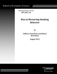
Figure A1. 

Figure A1: “Rescaling” of Likert Scale Responses 

Assume that respondents face a Likert scale with node values of 1, 1.5, 2, 2.5, 3, 

3.5 so the average of the scale values is 2.25. Because the distribution is symmetric, 

subjective distributions are rescaled and recentered around the values indicated. Anyone 

with a low assessment of their value for the characteristic, thinking she is out at the left 

30


tail, would assign herself a 1. A different person who believes she has to have an 

extremely high value of the characteristic gives herself a 4. Others with intermediate 

values move to the closest node. People between 3 and 3.25 move to 3, while those 

between 3.25 and 3.5 move to 3.5. In this case, the rounding errors offset; blue against 

red, purple against gray, green against orange, and the two halves of the yellow. The 

Likert scale provides an unbiased and consistent estimate of the mean value. The 

variance, however, is biased downward because the extreme values are not truncated. 

We note that if the location on the distribution is covariate dependent, then covariate 

analysis is biased because individual deviations persist. As already noted, the variance of 

the distribution of the characteristic is biased downward. 

Now suppose that some reason (for example, a bias against being associated with 

socially unacceptable behavior) keeps people from centering on the average of the Likert 

scale. In other words, the true distribution has a mean different from that offered by the 

Likert scale nodes. In terms of Figure 1, we can assume, for example, that the proffered 

Likert scale had nodes 1, 2, 3, and 4, with a mean value of 2.5, but the underlying 

distribution is as shown. Any respondent with a personal valuation below 1.5 assigns 

herself 1. Likewise, a respondent with a personal valuation above 3.5 assigns herself 4. 

Other intermediate values are likewise assigned to one of the integer nodes. Now, 

matching the colors we get a biased estimate of the mean, not just the variance. The blue 

and red areas together have an average value of 2.5, a bias of 0.25 above the mean. The 

purple and gray areas together have an average of 2, hence a bias of -0.25. Similarly, 

31


green and red have a bias of 0.25 when used to estimate the mean, and the yellow area 

has a bias of -0.25. As long as the distribution is not uniform the weighted average of 

these biases does not equal 0. For a normal distribution, as illustrated, the overall 

expected value is 2.33, an upward bias of 0.08. If the true mean is below the Likert mean 

the bias is upward. If the true mean is above the Likert mean the bias is downward. 

Obviously if the distribution is not symmetric a Likert scale will provide bias estimates of 

the mean, even when centered correctly. 

Finally, what does this imply for comparing pre- and post- treatment 

measurements? For a continuous distribution with infinite choices, moving any finite 

number of observations should not change the mean. In other words, unless the 

treatment is universally applied, there is no change in the average bias of the population. 

But, the treatment may shift, skew and/or alter the shape of the distribution of the 

selected sample, which is still measured with reference to the population distribution. 

Unless there are selection effects, the observations from the pre-treatment sample can 

be unbiased, but not the post-treatment observations, which now has a distribution 

different from the population distribution and more unbalanced than the original. People 

who were closer to the center of the distribution before the treatment still have a good 

chance of correctly showing their (positive) improvement. However, those who were 

near the (right) boundary have very little room to correctly show their improvement. 

Since the treatment pushes more people beyond the boundary, the measured treatment 

effect is always an underestimation. 

32


REFERENCES 

Abrevaya J, Hausman JA. 1999. Semiparametric Estimation with Mismeasured Dependent 

Variables: An Application to Panel Data on Employment Spells. Annales D'Economie et de 

Statistique 55-56: 243-75. 

Brossat DF, Clay DL, Willson VL. 2002. Methodological and Statistical Considerations for 

Threats to Internal Validity in Pediatric Outcome Data: Response Shift in Self-Report 

Outcomes. Journal of Pediatric Psychology 27(1): 97-107. 

Chua TC, Fuller WA. 1987. A Model for Multinomial Response Error Applied to Labor 

Flows. Journal of the American Statistical Association 82: 46-51. 

Cummins RA, Gullone E. 2000. Why we should not use 5-point Likert scales: The case for 

subjective quality of life measurement. Proceedings, Second International Conference on 

Quality of Life in Cities 74-93. Singapore: National University of Singapore. 

Dustmann C, van Soest A. 2000. Parametric and Semiparametric Estimation in Models 

with Misclassified Categorical Dependent Variables. IZA Discussion Papers no. 218. 

Hausman J. 2001. Mismeasured Variables in Econometric Analysis: Problems from the 

Right and Problems from the Left. The Journal of Economic Perspectives 15(4): 57-67. 

Hausman JA, Abrevaya J, Scott-Morton FM. 1998. Misclassification of the Dependent 

Variable in a Discrete-Response Setting. Journal of Econometrics 87: 239-269. 

Lewbel A. 2000. Identification of The Binary Choice Model with Misclassification. 

Econometric Theory 16(4): 603-609. 

33


Hill LG, Betz D. 2005. Revisiting the retrospective pretest. American Journal of Evaluation 

26: 501-517. 

Kruger J. 1999. Lake Wobegon be gone! The "below-average effect" and the egocentric 

nature of comparative ability judgments. Journal of Personality and Social Psychology 

77(2): 221-232. DOI: 10.1037/0022-3514.77.2.221 

Murphy, S. M., Rosenman, R., Yoder, J. K., & Friesner, D. L. 2011. Patient's perceptions 

and treatment effectiveness. Applied Economics DOI:10.1080/00036840903508395. 

Poterba JM, Summers LH. 1995. Unemployment Benefits and Labor Market Transitions: A 

Multinomial Logit Model with Errors in Classification. Review of Economics and Statistics 

77: 207-216. 

Rosenman R, Tennekoon V, Hill LG. Bias in Self Reported Data. International Journal of 

Behavioural and Healthcare Research forthcoming. 

Sprangers M, Hoogstraten J. 1989. Pretesting Effects in Retrospective Pretest-Posttest 

Designs. Journal of Applied Psychology 74(2): 265-272. 

Schwartz CE, Sprangers MAG. 1999. Methodological approaches for assessing response 

shift in longitudinal health-related quality-of-life research. Social Science & Medicine 48: 

1531-1548. 

34


Table 1: Determinants of Pr(y=1) with covariate dependant misclassification 

Variable 

True 

Value 

Probit HAS1 GHAS 

Est. Std. Err. Est. Std. Err. Est. Std. Err. 

α 

0 

= α 1 

=0.02 

Intercept -1.0 -0.913 0.049 -0.935* 0.079 -1.096** 0.206 

beta1 0.2 0.184 0.013 0.200*** 0.017 0.216* 0.027 

beta2 1.5 1.429 0.042 1.502*** 0.093 1.572** 0.160 

beta3 -0.6 -0.630** 0.070 -0.676* 0.093 -0.595*** 0.173 

α 

0 

= α 1 

=0.05 

Intercept -1.0 -0.793 0.048 -0.757 0.073 -1.106** 0.283 

beta1 0.2 0.162 0.015 0.186* 0.017 0.214** 0.032 

beta2 1.5 1.334 0.042 1.446* 0.088 1.570** 0.193 

beta3 -0.6 -0.679 0.072 -0.757 0.101 -0.568*** 0.246 

α 

0 

= α 1 

=0.1 

Intercept -1.0 -0.704 0.046 -0.642 0.119 -1.096*** 0.419 

beta1 0.2 0.128 0.014 0.174 0.023 0.214** 0.050 

beta2 1.5 1.033 0.039 1.252 0.139 1.562*** 0.330 

beta3 -0.6 -0.454 0.069 -0.580*** 0.114 -0.580*** 0.347 

α 

0 

= α 1 

=0.2 

Intercept -1.0 -0.562 0.044 -1.402* 0.432 -1.132*** 0.537 

beta1 0.2 0.088 0.013 0.265* 0.090 0.224** 0.086 

beta2 1.5 0.754 0.037 1.758** 0.519 1.587*** 0.511 

beta3 -0.6 -0.145 0.064 -0.517** 0.288 -0.551*** 0.526 

α 

0 

=0.02 , α 

1 

=0.2 

Intercept -1.0 -0.924 0.049 -0.842 0.100 -1.152** 0.344 

beta1 0.2 0.131 0.016 0.207** 0.027 0.221** 0.044 

beta2 1.5 1.140 0.041 1.467** 0.156 1.593** 0.270 

beta3 -0.6 -0.631** 0.069 -0.841 0.136 -0.563*** 0.344 

α 

0 

=0.2 , α 

1 

=0.02 

Intercept -1.0 -0.563 0.044 -1.349 0.282 -1.085** 0.334 

beta1 0.2 0.135 0.011 0.229* 0.047 0.217** 0.041 

beta2 1.5 1.077 0.039 1.685* 0.280 1.574** 0.266 

beta3 -0.6 -0.152 0.066 -0.351 0.162 -0.600*** 0.248 

*** True value is within 0.25 standard deviations from the estimate. 

** True value is within 0.5 standard deviations from the estimate. 

* True value is within 1 standard deviation from the estimate. 

35


Table 2: Determinants of Pr(yo=1|y=0) with covariate dependant 

misclassification 

Variable 

True 

Value 

HAS1 

Est. 

Std. 

Err. 

GHAS 

Est. 

Std. 

Err. 

α 

0 

= α 1 

=0.02 

Intercept -1.50 -1.388*** 0.834 

gamma01 -1.44 -3.365** 5.350 

α 

0 

0.02 0.009* 0.015 

α 

0 

= α 1 

=0.05 

Intercept -1.00 -0.890** 0.234 

gamma01 -1.64 -4.500*** 32.107 

α 

0 

0.05 0.003 0.008 

α 

0 

= α 1 

=0.1 

Intercept -1.00 -1.470*** 4.810 

gamma01 -0.60 -0.518*** 5.053 

α 

0 

0.10 0.014 0.026 

α 

0 

= α 1 

=0.2 

Intercept -1.00 -1.438*** 2.473 

gamma01 0.31 0.651*** 2.536 

α 

0 

0.20 0.222** 0.066 

α 

0 

=0.02 , α 

1 

=0.2 

Intercept -1.50 -1.397*** 1.212 

gamma01 -1.44 -28.221*** 354.692 

α 

0 

0.02 0.011* 0.017 

α 

0 

=0.2 , α 

1 

=0.02 

Intercept -1.00 -1.072*** 0.599 

gamma01 0.31 0.379*** 0.545 

α 

0 

0.20 0.225* 0.050 




36


Table 3: Determinants of Pr(yo=0|y=1) with covariate dependant misclassification 

Variable 

True 

Value 

HAS1 

GHAS 

Est. Std. Err. Est. Std. Err. 

α 

0 

= α 1 

=0.02 

Intercept -1.50 -1.822*** 2.209 

gama11 -0.20 -0.394*** 2.765 

gama12 -1.20 -14.147*** 125.833 

α 

1 

0.02 0.025*** 0.025 

α 

0 

= α 1 

=0.05 

Intercept -1.00 -1.329*** 1.326 

gama11 -0.26 -0.006*** 1.487 

gama12 -1.20 -4.006*** 13.245 

α 

1 

0.05 0.061** 0.040 

α 

0 

= α 1 

=0.1 

Intercept -1.00 -1.422** 1.102 

gama11 0.24 0.627** 1.076 

gama12 -0.72 -1.219*** 2.836 

α 

1 

0.10 0.133* 0.057 

α 

0 

= α 1 

=0.2 

Intercept -1.00 -1.474** 1.054 

gama11 0.15 0.436** 0.989 

gama12 0.12 0.190*** 0.891 

α 

1 

0.20 0.205** 0.072 

α 

0 

=0.02 , α 

1 

=0.2 

Intercept -1.00 -1.360** 1.096 

gama11 0.15 0.449** 1.081 

gama12 0.12 0.054*** 0.834 

α 

1 

0.20 0.208*** 0.055 

α 

0 

=0.2 , 

1 

α =0.02 

Intercept -1.50 -3.109*** 15.855 

gama11 -0.20 -0.282*** 2.269 

gama12 -1.20 -7.522*** 35.332 

α 

1 

0.02 0.025*** 0.028 




37


Table 4: Determinants of Pr(y=1) when the misclassification probabilities are constants 

Variable 

True 

Value 


Est. 

Std. 

Err. Est. 

Std. 

Err. Est. Std. Err. 

α 

0 

= α 1 

=0.02 

Intercept -1.0 -0.939 0.048 -1.044** 0.128 -1.128* 0.239 

beta1 0.2 0.183 0.014 0.208** 0.023 0.220* 0.030 

beta2 1.5 1.407 0.043 1.542** 0.137 1.590** 0.188 

beta3 -0.6 -0.547* 0.071 -0.624*** 0.109 -0.579*** 0.212 

α 

0 

= α 1 

=0.05 

Intercept -1.0 -0.852 0.049 -1.031*** 0.164 -1.098** 0.293 

beta1 0.2 0.160 0.014 0.207*** 0.032 0.215** 0.038 

beta2 1.5 1.285 0.042 1.531*** 0.184 1.576** 0.245 

beta3 -0.6 -0.485 0.072 -0.619*** 0.139 -0.591*** 0.267 

α 

0 

= α 1 

=0.1 

Intercept -1.0 -0.729 0.046 -1.019*** 0.206 -1.079*** 0.384 

beta1 0.2 0.131 0.014 0.203*** 0.039 0.210*** 0.047 

beta2 1.5 1.108 0.039 1.506*** 0.235 1.546*** 0.326 

beta3 -0.6 -0.400 0.070 -0.604*** 0.160 -0.571*** 0.369 

α 

0 

= α 1 

=0.2 

Intercept -1.0 -0.516 0.045 -1.057*** 0.344 -1.123*** 0.616 

beta1 0.2 0.086 0.013 0.212*** 0.064 0.224** 0.089 

beta2 1.5 0.793 0.037 1.550*** 0.389 1.583*** 0.549 

beta3 -0.6 -0.266 0.067 -0.617*** 0.234 -0.541*** 0.568 




. 

38


Table 5: Determinants of Pr(yo=1|y=0) when the misclassification 

probabilities are constants 

Variable 

True 

Value 

HAS1 

Est. 

Std. 

Err. 

GHAS 

Est. 

Std. 

Err. 

α 

0 

= α 1 

=0.02 

Intercept -2.05 -2.329*** 2.236 

gamma01 0.00 -0.215*** 3.016 

α 

0 

0.02 0.028** 0.026 

α 

0 

= α 1 

=0.05 

Intercept -1.64 -2.080*** 1.967 

gamma01 0.00 0.035*** 3.030 

α 

0 

0.05 0.052*** 0.036 

α 

0 

= α 1 

=0.1 

Intercept -1.28 -1.651** 1.370 

gamma01 0.00 0.074*** 2.269 

α 

0 

0.10 0.093*** 0.047 

α 

0 

= α 1 

=0.2 

Intercept -0.84 -1.157** 1.163 

gamma01 0.00 0.135*** 1.109 

α 

0 

0.20 0.188*** 0.068 




39


Table 6: Determinants of Pr(yo=0|y=1) when the misclassification 

probabilities are constants 

HAS1 

GHAS 

Variable 

True 

Value 

Est. 

Std. 

Err. 

Est. 

Std. 

Err. 

α 

0 

= α 1 

=0.02 

Intercept -2.05 -28.029*** 342.046 

gama11 0.00 -0.970*** 12.358 

gama12 0.00 -24.089*** 354.267 

α 

1 

0.02 0.023*** 0.024 

α 

0 

= α 1 

=0.05 

Intercept -1.64 -2.312** 1.595 

gama11 0.00 0.324*** 1.737 

gama12 0.00 -2.729*** 21.886 

α 

1 

0.05 0.050*** 0.035 

α 

0 

= α 1 

=0.1 

Intercept -1.28 -1.789** 1.204 

gama11 0.00 0.217*** 1.430 

gama12 0.00 -2.045*** 21.213 

α 

1 

0.10 0.089*** 0.050 

α 

0 

= α 1 

=0.2 

Intercept -0.84 -1.180** 0.925 

gama11 0.00 0.189*** 0.939 

gama12 0.00 0.067*** 1.013 

α 

1 

0.20 0.186*** 0.070 




40


Table 7: Variable Names, Descriptions and Summary Statistics 

Name Description Mean Std. Dev. 

Improved 

Observed (misclassified) binary dependant 

variable: Equal to 1 if post-test score > pre-test 

score 

0.708 0.455 

Male Equal to 1 if the gender is reported as male; 0 

otherwise 0.250 0.433 

Gender Not Reported Equal to 1 if the gender is not reported; 0 

otherwise 

Black/African American 

0.030 0.170 

Equal to 1 if the race is reported as African 

American; 0 otherwise 0.023 0.150 

Hispanic/Latino Equal to 1 if the race is reported as Hispanic; 0 

otherwise 

Native American 

Other Races 

Race Not Reported 

0.269 0.443 

Equal to 1 if the race is reported as Native 

American; 0 otherwise 0.040 0.195 

Equal to 1 if the race is reported as other or of 

multiple ethnicity; 0 otherwise 

Equal to 1 if the race is not reported; 0 otherwise 

0.034 0.182 

0.034 0.182 

Age Integer (17-73) 38.822 7.846 

Living with Partner or Equal to 1 if reported living with partner or 

spouse 

spouse; 0 otherwise 

0.736 0.441 

Partner/Spouse Details Not 

Reported 

Program Average of Prescore 

Program Std. Dev. of Prescore 

Pre-test Score 

Equal to 1 if the partner/spouse details not 

reported; 0 otherwise 

Average of the pre-scores of the participants 

enrolled in the same program; Continuous 

variable between 1-5 

Standard deviation of the pre-scores of the 

participants enrolled in the same program; 

Continuous variable 

Self-reported pre-test score; Semi-continuous 

variable between 1-5 

0.077 0.266 

3.987 0.237 

0.499 0.173 

3.979 0.546 

Pre-test Score > 4.9 Equal to 1 if the pre-score > 4.90; 0 otherwise 0.033 0.178 

41


Table 8: Determinants of True Improvement in Family Functionality 

Variable 


Est. 

Std. 

Err. Est. 

Std. 

Err. Est. 

Improvement 

Male -0.250 *** 0.090 -0.300 *** 0.103 0.572 0.517 

Gender Not Reported 0.436 0.305 0.548 0.403 -2.032 *** 0.786 

Excluded: Female 

Black or African-American -0.525 ** 0.239 -0.563 ** 0.252 -0.368 0.744 

Hispanic -0.148 0.096 -0.120 0.111 1.139 * 0.680 

Native American -0.294 0.194 -0.319 0.213 -0.424 0.735 

Other Races -0.115 0.201 -0.052 0.241 3.166 6.290 

Race Not Reported 0.375 0.290 0.357 0.326 -1.441 * 0.827 

Excluded: White 

Age -0.002 0.005 -0.003 0.006 -0.015 0.022 

Living with Partner/Spouse -0.158 0.105 -0.162 0.118 1.151 *** 0.402 

Partner/Spouse Details Not 

Reported -0.500 *** 0.166 -0.573 *** 0.187 2.367 *** 0.832 

Excluded: Not Living with 

Partner/Spouse 

Program Average of Pre-score 0.165 0.199 0.307 0.241 1.568 ** 0.762 

Program Std. Dev. of Pre-score -0.337 0.250 -0.225 0.296 2.029 ** 1.023 

Pre-score -1.358 *** 0.096 -1.612 *** 0.173 1.454 *** 0.440 

Intercept 5.951 *** 0.834 6.527 *** 1.060 -12.635 *** 3.387 

*** p


Table 9: Determinants of Probabilities of Misclassification 

Variable 

HAS1 

Est. 

Std. 

Err. 

GHAS 

Recording No Improvement as Improvement 

Black or African-American -7.831 5.534 

Hispanic -15.193 * 9.007 

Race Not Reported and other races -3.317 4.032 


Age 0.629 * 0.358 

Pre-score -3.922 * 2.088 

Intercept 2.849 5.747 

α 

0 

0.000 *** 0.000 

Recording Improvement as No Improvement 

Black or African-American 0.428 0.368 

Hispanic -0.143 0.137 

Race Not Reported and other races 0.149 0.202 


Age 0.013 * 0.007 

Pre-score 1.139 *** 0.146 

Pre-score > 4.9 1.086 *** 0.355 

Intercept -5.533 *** 0.702 

α 

1 

0.0320 0.020 

*** p

Systematically Misclassified Binary Dependant Variables

Create successful ePaper yourself

Delete template?

Save as template?