3.04 Gravimetric Methods – Superconducting Gravity Meters

78 Superconducting Gravity Meters
type of material (clay, gravel, sand, etc.) will play an
important factor in the interpretation of meteorological
and other seasonal effects. For example, it has been
found that porous material can compress and deform
under loading and thus generate an unwanted signal.
Whatever the height of the SG with respect to the
local ground level, an important factor effect is the soil
moisture content of the local and regional area from 1
to 100 m around the gravimeter. Soil moisture resides
largely in a layer no more than 1 or 2 m thick, but the
effect on an SG can be significant. Installation of
groundwater sensors, soil moisture probes, rainfall
gauge, and other meteorological sensors are required
for developing advanced hydrological models at the
sub-mGal level.
The requirements of location, site noise, and site
preparation need to be assessed very carefully by
potential new users. Considerable experience lies
both with the manufacturer (GWR) and with many
experienced SG owners, who have maintained their
stations for a decade or longer. Although there is no
central funding source for establishing new SG sites,
potential new users are encouraged to contact existing
SG groups for advice, particularly through the
GGP website, GGP workshops, and by visiting operating
GGP sites.
tilts). The gravity is typically recorded at 1, 2, or 5 s
intervals, whereas the auxiliary signals are often
sampled at lower rates, for example, 1 min.
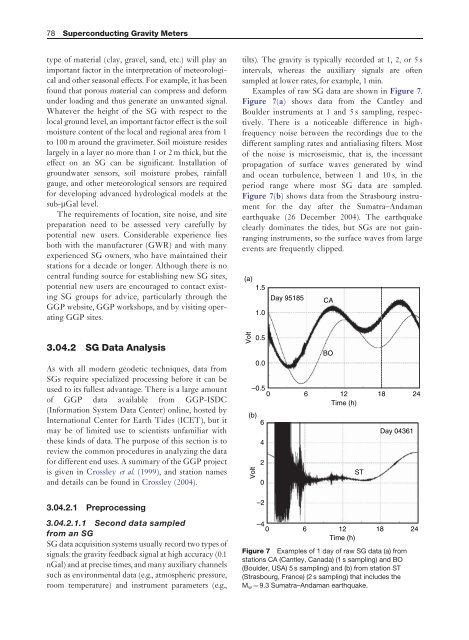
Examples of raw SG data are shown in Figure 7.
Figure 7(a) shows data from the Cantley and
Boulder instruments at 1 and 5 s sampling, respectively.
There is a noticeable difference in highfrequency
noise between the recordings due to the
different sampling rates and antialiasing filters. Most
of the noise is microseismic, that is, the incessant
propagation of surface waves generated by wind
and ocean turbulence, between 1 and 10 s, in the
period range where most SG data are sampled.
Figure 7(b) shows data from the Strasbourg instrument
for the day after the Sumatra–Andaman
earthquake (26 December 2004). The earthquake
clearly dominates the tides, but SGs are not gainranging
instruments, so the surface waves from large
events are frequently clipped.
(a)
1.5
Day 95185
1.0
CA
3.04.2 SG Data Analysis
As with all modern geodetic techniques, data from
SGs require specialized processing before it can be
used to its fullest advantage. There is a large amount
of GGP data available from GGP-ISDC
(Information System Data Center) online, hosted by
International Center for Earth Tides (ICET), but it
may be of limited use to scientists unfamiliar with
these kinds of data. The purpose of this section is to
review the common procedures in analyzing the data
for different end uses. A summary of the GGP project
is given in Crossley et al. (1999), and station names
and details can be found in Crossley (2004).
3.04.2.1 Preprocessing
Volt
0.5
0.0
BO
–0.5
0 6 12
Time (h)
(b)
6
Volt
4
2
0
–2
ST
18 24
Day 04361
3.04.2.1.1 Second data sampled
from an SG
SG data acquisition systems usually record two types of
signals: the gravity feedback signal at high accuracy (0.1
nGal) and at precise times, and many auxiliary channels
such as environmental data (e.g., atmospheric pressure,
room temperature) and instrument parameters (e.g.,
–4
0 6 12
Time (h)
18 24
Figure 7 Examples of 1 day of raw SG data (a) from
stations CA (Cantley, Canada) (1 s sampling) and BO
(Boulder, USA) 5 s sampling) and (b) from station ST
(Strasbourg, France) (2 s sampling) that includes the
M w ¼ 9.3 Sumatra–Andaman earthquake.