3.04 Gravimetric Methods – Superconducting Gravity Meters

96 Superconducting Gravity Meters
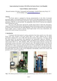
compact SG, in this case the C012 at Membach. The
electronic step was applied to various combinations
of filter type and time intervals (1–4 min), and the
output was Fourier-analyzed to determine the amplitude
and phase response. The time lag results showed
an accuracy of 0.003 s for the GGP1 filter and
0.075 s for the raw gravity signal output. The sine
wave method gave very similar results, confirming
the integrity of the method. The amplitude gain of
the electronics system was determined to be flat
from 500 to 2000 s, the longest period determined
by either method. Further details are given on the
GGP website.
3.04.2.5 Other Corrections to Residual
Gravity
3.04.2.5.1 Polar motion
One important signal contained in an SG record is
the 14 month (435 day) oscillation of the rotation
pole, or Chandler wobble. As noted previously,
Richter’s (1983) first observation of this signal, with
only 5 mGal amplitude, was a turning point in the
refinement of gravity residuals. Since then, every SG
station has recorded data that when suitably processed
show the polar motion (e.g., Harnisch and
Harnisch, 2006a). Naturally, some records are very
clear and others not so clear, depending on the epoch
(amplitude of the motion) and the quality of the
instrument and site.
With most data sets, it is not difficult to see the
polar motion once tides and atmospheric pressure are
subtracted. Indeed, for the most part, the highly
accurate space geodetic series for the polar orientation
that is given on the IERS website can be used
directly at any of the gravity stations. A simple conversion
is usually made between the (x, y) amplitudes
of polar motion (m 1 , m 2 ) in radians and the gravity
effect g in mGal (e.g., Wahr, 1985):
g ¼ 3:90 10 9 sin 2 ½cosðm 1 Þ sinðm 2 ÞŠ ½6Š
where (,) are station latitude and longitude. The
numerical factor includes the nominal value of 1.16
for the gravimetric delta factor, whereas fitted solutions
are usually closer to ¼ 1.18 (e.g., Loyer et al.,
1999; Harnisch and Harnisch, 2006b). In many studies,
the polar motion is considered as a quantity very
accurately determined from space geodetic data, but
it is interesting to observe its signature in either an
individual or collective gravity series.
3.04.2.5.2 Instrument drift
From a historical viewpoint, particularly for spatial
gravity surveys, the term ‘drift’ has been applied to
almost any unwanted time-varying gravity signal.
This usage persists in the SG literature and sometimes
causes confusion. Here we use drift as an
instrument characteristic, because all other gravity
variations have specific causes.
From an instrumental point of view (e.g.,
Goodkind, 1999), drift is likely to be either a linear
or exponential function of time, but its size is not easy
to predict. The exponential behavior can be reset
after a loss of levitation or other magnetic changes
within the sensor. Under normal operation, the user
can generally assume that drift will level off after
installation and gradually become more linear as
time progresses. Representative values of instrument
drift are frequently less than 4 mGal yr 1 where these
have been checked carefully with AGs (see above).
From a processing point of view, other functions
such as polynomials have been used as a model for
instrument drift but there is no physical reason to
prefer such a choice. We recommend that an exponential
drift be assumed from some initialization
event for the instrument and later this may be
replaced with a simple linear function. Drift is not
to be confused with a secular change of gravity, even
though the two cannot be separated except using
combined SG–AG observations.
3.04.2.5.3 Hydrology
Hydrology is perhaps the most complex of the intermediate
scale (hour–year) variations in gravity (e.g.,
Harnisch and Harnisch, 2006a). This is due to two
factors. The first is its variability, due largely to the
local water storage balance at the station that
involves many components (rain and snowfall, soil
moisture, evapotranspiration, and runoff ). Rainfall is
relatively easy to assess, as is the groundwater level,
which is usually measured in a nearby well. The
direct measurement of soil moisture is not easy and
has not been done at most SG stations.
The second problem is one of length scales. The
connectedness (permeability) of the soils and
groundwater system is inhomogeneous at the local
length scales (meter to kilometers), and so an assessment
of the amount of moisture surrounding an SG
involves extensive measurements. This quantity predominantly
affects the attraction term rather than the
loading term.
As a result, even though groundwater variations
are extremely useful, they are not entirely reliable for