3.04 Gravimetric Methods – Superconducting Gravity Meters
3.04 Gravimetric Methods – Superconducting Gravity Meters
3.04 Gravimetric Methods – Superconducting Gravity Meters

You also want an ePaper? Increase the reach of your titles
YUMPU automatically turns print PDFs into web optimized ePapers that Google loves.
92 <strong>Superconducting</strong> <strong>Gravity</strong> <strong>Meters</strong><br />
Europe over a 2 year period (only the annual fitted<br />
function is shown). In the summer months, the air<br />
masses within the atmosphere rise and the gravitational<br />
attraction effect decreases (upward); this causes a net<br />
positive gravity effect at the ground that is about 1 mGal<br />
larger than that in winter months. Neumeyer et al.<br />
(2004a) showed that the effect is not the smooth function<br />
shown in Figure 13(c), buttherearesudden<br />
changes that occur over periods of days. The computational<br />
effort to include this term is not trivial and it is<br />
being done routinely only at a few SG stations; one<br />
limitation is the need to interpolate the meteorological<br />
data that is available only at 6 h sampling and 0.5 <br />
(50 km) spacing. This is also a factor for the data reduction<br />
in GRACE because the atmospheric pressure<br />
corrections are done on the inter-satellite distance<br />
timescales that are aliased by 6 h sampling.<br />
<strong>3.04</strong>.2.4 Calibration Issues<br />
<strong>3.04</strong>.2.4.1 Basics<br />
SGs are relative instruments and no ‘factory calibration’<br />
is provided by the manufacturer. The instrument must<br />
be calibrated to convert its output feedback voltage, as<br />
recorded by a digitizing voltmeter, to units of acceleration.<br />
The amplitude calibration factor (GCAL) is<br />
frequently called the scale factor of the instrument and<br />
is expressed in mGal V 1 or nm s 2 V 1 , with a typical<br />
value of about 80 mGal V 1 (Table 5). In addition, the<br />
system transfer function of the complete system (sensor<br />
and electronics) must be measured to determine the<br />
frequency dependence of both the amplitude and<br />
phase. Although it is easy to find the approximate calibration<br />
(to a few % in amplitude or phase), it is<br />
nontrivial to improve the calibration to be better than<br />
0.1%. There are three applications for which accurate<br />
calibration is most important: (1) ocean tide loading or<br />
solid Earth tidal deformation including the FCN resonance,<br />
(2) the subtraction of a synthetic model for tides<br />
and the atmosphere whenever residuals are required to<br />
high accuracy, and (3) for determining precise spectral<br />
amplitudes in normal-mode studies.<br />
The SG output has a very large bandwidth, from<br />
1 s (the raw sampling) to periods as long as the data<br />
length (years to decades). It is common to refer to the<br />
long period limit as ‘DC’ (vaguely meaning beyond<br />
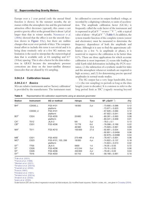
Table 5<br />
Representative SG calibration experiments using an absolute gravimeter<br />
Station Instrument AG or method #drops Time SF (mGal V 1 ) (%)<br />
BH a CD030_L FG5 #101 18 000 2 yr 73.690 0.088 0.12<br />
platform 73.971 0.023 0.03<br />
CD030_U FG5 #101 67.626 0.084 0.12<br />
platform 67.922 0.041 0.06<br />
BO b C024 FG5 #205 20 800 9 d 80.281 0.063 0.08<br />
platform 80.341 0.009 0.01<br />
CA c T012 JILA-2 NA 3 yr 78.3 0.1 0.13<br />
CB d C031 FG5 #206 15 778 6 d 76.098 0.169 0.22<br />
46 560 12 d 75.920 0.061 0.08<br />
MA e T011 FG5 #210 100 000 27 d 92.801 0.034 0.04<br />
92.851 0.049A 0.06<br />
92.879 0.036B 0.04<br />
MB f C021 FG5 #202 275 468 47 d 78.457 0.001 0.06<br />
MC g C023 FG5 #101, 103, 206 18 000 4 yr 74.822 0.137 0.18<br />
platform 74.824 0.013 0.02<br />
ST h TT05 JILA-5 5600 1 d 76.05 0.55 0.72<br />
ST i C026 FG5 #206 412 244 3 yr 79.19 0.05 0.06<br />
ST j C026 FG5 #206 450 000 4 yr 79.40 0.03 0.04<br />
SY k T016 FG5 #203 55 743 15 d 58.168 0.061 0.10<br />
a Falk et al. (2001);<br />
b Francis et al. (1998);<br />
c Merriam et al. (2001);<br />
d Amalvict et al. (2001b);<br />
e Imanishi et al. (2002);<br />
f Francis (1997);<br />
g Hinderer et al. (1991);<br />
h Amalvict et al. (2001a);<br />
i Amalvict et al. (2002);<br />
j Iwano et al. (2003).<br />
Scale factors (SF) are by direct regression except (a) tidal analysis, (b) modified least squares. Station codes, etc., are given in Crossley (2004).