SPCImage 4.0 - Becker & Hickl

Becker & Hickl GmbH February 2013
High Performance
Photon Counting
Tel. +49 - 30 - 787 56 32
FAX +49 - 30 - 787 57 34
http://www.becker-hickl.com
email: info@becker-hickl.com
SPCImage 4.0
Data Analysis Software for
Fluorescence Lifetime Imaging Microscopy
New features:
♦ Batch processing of freely selectable data files
♦ Intensity overlay by fit parameters
♦ Definition of multiple ROIs
♦ Improved zoom functions
♦ Automatic background suppression
♦ Enhanced calculation speed

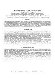
1. Introduction
SPCImage was designed to analyse data of fluorescence lifetime imaging measurements (FLIM)
by fitting them to a “model”. The approach is to minimize the chi-square value between the
data and the model function during the fit process. The result is a set of parameters ( e.g.
lifetimes ) for each individual pixel of the image. In a subsequent step the user selects one of
the parameters or a mathematical combination of different parameters to create a “lifetime
image”.
The time slope of the fluorescence follows an exponential behavior if the transfer rate which
depletes the excited state is a constant in time. This holds true for all experiments which use
moderately low intensities far away from the threshold of stimulated emission. However, there
are several effects which make the definition of the model function more complicated. Two of
them are:
i) The fluorescence which originates from one pixel can be an overlay of the emissions of
different chromophores.
ii)
The chromophores within a single pixel of the FLIM image are in different
photophysical states (e.g. due to changes in the microenvironment or energy transfer
processes ).
log I
log I
F(t) =
-t /
a e 1
1
+
-t /
a e 2
2
-t /
a e
1
1
-t /
a e 2
2
time
time
Figure 1: Sum of two exponential decays showing different lifetimes
2

The time slope of a fluorescence decay in a lifetime image usually is a sum of different
exponential decays. With up to three different components the model function for each
individual pixel runs as:
F(
t)
−t
/ τ1 −t
/ τ 2 −t
/ τ 3
= a e + a e + a e
(1)
1
2
3
It is up to the user how many exponential components are selected. Measurements with quite
poor signal-to-noise ratios (SNR), i.e. a low number of photons per pixel might allow a single
exponential model. In this case the amplitude coefficients a 2 and a 3 are set to zero. However, in
cases in which the fluorescence was measured with a good SNR the user will have to switch to
a double exponential decay or even go up to three exponential components.
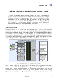
Equation (1) is valid if the width of the instrumental response function (IRF) of the
measurement system is small compared to the width of the time channels of the histogram in
which the photons are stored. The IRF defines the overall time-resolution of the measurement
system. It is defined by the pulse-width of the laser ( which is negligible small for a femtosecond
laser system ), the electrical resolution of the measurement system and ( most important ) the
time resolution of the detector. In a typical experiment ( fast lifetimes, small channel-width) the
measured intensity follows a convolution of the model function F(t) and the instrumental
response function R(t).
I
(
S
t)
= F ( t)
⊗ R(
t − t )
(2)
log I
R(t)
log I
I(t) =
R(t)
⊗ F(t)
F(t) =
-t /
a e
time
time
Figure 2: Convolution of an instrumental response function R(t) with a single exponential decay trace
3

Here the calculated function which is fitted to the decay trace is an integral over time.
SPCImage provides an “estimation” of this response function by calculating the first derivative
of the rising part of the fluorescence. However, it is preferable to determine this function by an
experiment. The parameter t S denotes a linear shift between the reponse function and the
fluorescence and is determined automatically by the software.
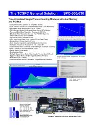
Another complication can arise due to scattered light or a second harmonic light generation
inside the sample which bleeds into the detection channel causing a pronounced peak in the
first part of the curve.
~
I ( t)
= I ( t)
+ s ⋅ R(
t)
(3)
log I
log I
I(t)
I(t)+
s R(t)
s R(t)
time
time
Figure 3: Effect of scattering or fluorescence bleedthrough
Since the scattering and/or second harmonic generation processes R(t) are extremely fast
compared to the response time of the system it adds linearly to the decay trace I(t) with a factor
s =“scatter” which can be defined as a fitting parameter.
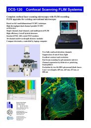
In addition almost all detection systems pick up some ambient (room) light which together with
the noise of the detector produces a constant baseline or “offset”. This number has to be taken
into account to avoid the artificial generation of a long-lifetime component by the fitting
process. The “offset” a 0 can either be measured by an independent dark experiment or
determined automatically by means of the photons which are in the time channels in front of
the rising part of the fluorescence decay trace. However, in addition to the dark noise of the
detector also the effect called “afterpulsing” contributes to the noise. Since afterpulsing
depends on the countrate of the detector it is not possible to derive it from a dark experiment.
4

Please make sure the measurement control parameters and cable-length are selected
accordingly to get enough time channels into this “pre-curve” part.
Offsetcalculation
I(t)
log I
~
I(t) =
I(t) + a
0
a 0
time
time
Figure 4a: Effect of ambient light and detector dark noise
The “Incomplete Model” should be used if the fluorescence decay is slow compared to the time
window which is defined by the repetition rate of the laser system. If the time between the
exciting laser pulses is given as an input parameter the software calculates the amount of
fluorescence which arises from all previous laser-pulses. The most significant contribution is
from the laser period which is located directly before the current one as shown in fig. 4b.
I(t)
Previous Laser Pulse
Current Laser Pulse
time
Figure 4b: Effect of “incomplete decay” on the fluorscence decay
The situation gets more complicated if there is a constant offset due to ambient light or
afterpulsing. SPCImage can only perform a rough approximation between offset correction and
incomplete decay contribution.
5

2. Analyzing fluorescence lifetime images
SPCImage provides access to the “lifetime information” of a time- and spatially resolved
dataset which was measured with one of the TCSPC imaging boards from bh. There are two
ways to transfer the data from the measurement software SPCM to SPCImage: DDE-transfer
and sdt file import. The DDE transfer can be invoked by Send Data to SPC-Image in the
measurement software. File import can be done by File>Import in SPCImage.
The TCSPC package on CD/DVD contains several sample data files which can be found in the
“\Datafiles” directory. An intensity image is displayed after successfully importing the “cells.sdt”
file.
Intensity Image
Region of Interest:
(lower left corner)
Region of Interest:
(upper right corner)
„Hot spot“
Defines a pixel from
which the current
decay trace is shown
Figure 5: Image which is shown after importing the cell.sdt file
SPCImage uses auto-scaling to select the intensity scale of an image. In case this method
produces unsatisfactory results the scale can be changed manually ( see Options > Intensity
dialog in section 3 ).
After loading the data SPCImage will choose the brightest pixel of the image as a “Hot spot”.
The location is indicated by the blue crosshair and a numerical position (x,y) is given in the
decay window as described below. The IRF is estimated from the data trace which belongs to
the selected pixel.
Pixel selection can be changed by moving the blue crosshair. Please invoke the IRF>Auto
command to repeat the estimation of the IRF for the currently selected.
6

Two white crosshairs are located in the upper right and lower left corner of the image defining
a region of interest (ROI) which will be used for data analysis. They can be changed by clicking
on the white dots and moving them to a different location. Thus, object(s) in the image can be
selected by defining a “box” around them. Please note: Defining ROIs may save computation
time as only the area inside the crosshairs is calculated.
The “Decay-Graph” is located beneath the intensity image and contains several numerical
parameters. The following items are shown: The photon decay data ( blue ), trace of the fit
T1: Start of fit (channel number)
T2: End of fit (channel number)
Spatial binning
Threshold
Position of
selected pixel
Selected fit
parameter
( red ) and the response function ( green ).
Reduced chi-square
Response function
Measured decay trace
(dotted) and fit curve
(line)
Weighted
residuals
Sum of
photons
Figure 6: Decay graph which is shown after importing the cell.sdt file
Deviations between photon data and fit-trace are represented by the weighted residuals at the
bottom. It is important to define a range of time channels to improve the quality of the fit. Start
and end position of this range are given numerically by the T1 and T2 values ( time channels ).
Please note that only data-points between the two vertical black cursor lines are used for the fit
process.
7

By default all time channels in front of the first cursor line ( i.e. channels 0 to T1-1 ) are used for
calculating the baseline or “offset” as indicated in the introduction. Since the calculation of the
offset is very important in order to receive correct lifetimes it is recommended to shift the rising
part of the fluorescence to about 1/10 th of the complete range to have enough data points in
front of fluorescence decay .
The Binning factor denotes the number of surrounding pixels which are summed into each
decay trace:
The number of photons in each decay trace will increase effectively if the binning value is
incremented. However, the spatial resolution will decrease since the binning strategy is used for
all the pixels within the region of interest during the fit process. Please adjust the binning factor
in according to the signal-to-noise ratio of your measurement.
As a rule of thumb the peak value of the curve should be at least 100 for a single exponential
fit, about 1000 for a double-exponential decay and 10000 for three exponentials. This holds
true for situations where all lifetimes are unknown. The required number of photons will be
decreased if there is any a priori knowledge of a lifetime which can be use to “fix” one or more
values
Binning
(2n+1)x(2n+1)
area
n
0
1
2
3
Figure 7: Binning mehtod and dependency on the binning-factor “n”
The Threshold-parameter defines the minimum required number of photons in the peak of a
fluorescence curve. By default the threshold parameter is auto-adjusted to suppress all pixels
with a peak fluorescence smaller than 20% of the average. This is to accelerate the calculation
process and for improving the quality of the parameter histogram ( see below ) since outliers
due to a bad signal-to-noise ratio will be suppressed. The Threshold-parameter can also be
changed manually ( see Options > Model dialog in section 3 ).
8

To start the image analysis within a selected ROI the Calculate>Decay Matrix command is
used. During the process of calculating the decay matrix the region of interest is analysed pixel
by pixel and line by line. The following figure shows the situation if the binning-factor is set
to 1.
Matrix of measurement data
3 3 1 3 1 4 3 1 4 1 3 1 4 1 5
Matrix of calculated fit parameters
Figure 8: Sequence of calculation of the fit parameters
A color coded lifetime image will be shown after calculation was finished. This image derives
the intensity information from the number of photons in each pixel and the color information
from a selected fit parameter which value is coded by a continuous color scale.
Figure 9: Result of performing the Calculate>Decaymatrix command wihtin a defined ROI
A histogram shows the distribution of the parameter which is currently selected (tm, default).
On x-axis the selected parameter value is plotted whereas y-axis denotes the number of pixels
in which the value was found.
9

If the intensity window is hidden by disabling the Options>Preferences: Show Intensity
Window- checkbox the histogram window will be displayed enlarged ( Figure 10 ).
If – in addition – the Options>Preferences: Show Intensity in Lifetime Window
checkbox is selected the images of both windows are merged. Please note: In black and white
regions no analysis was performed.
Figure 10: Combined presentation of lifetime & intensity image and detailed distribution histogram
The software determines the mean value of the distribution µ and marks it by the small white
crosshair. In addition the standard deviation µ ± σ is calculated and displayed by two white
vertical cursor lines.
The distribution can be switched to “weighted” in order to multiply the lifetime frequencies
with the corresponding number of photons in each pixel ( see Options > Preferences in section
3 ).
Color range is auto-scaled by default to cover most of the parameter values. The scale cane be
changed to user settings in Options>Color dialog by means of the “Range: Min/Max “-
values. It is also possible to reverse color scaling or use an “RGB” color-coding with discrete
ranges ( see Options > Color in section 3 ).
Next to the residual plot the reduced χ 2
the quality of the fit. It is defined as
as denoted in the decay graph can be used to check
N
2
2 1 ( di
− fi
)
r
= ∑
N − p i=
1 di
χ (4)
10

3. Menu commands
File → Import
SPCImage gets fluorescence lifetime data from the measurement software SPCM. Therefore it
is necessary to transfer data between the two applications. The dataset from the SPC module
can be loaded into the application by importing an .sdt file which was previously created by the
measurement software. In addition it is possible to load-in ASCII datafiles or invoke a direct
data transfer from the measurement software ( Send Data to SPCImage -> see chapter 2 ).
On selecting an “.sdt”-File a dialog window shows a brief summary of the measurement
information stored in the .sdt file. The identification part is shown on the left. It contains
information about the version of the acquisition software, the time and date of the
measurement and a comment line eventually contained in the data file.
The size of the image, number of time channels and other measurement parameters are given
at the right side of the dialog.
The Count Increment denotes how the histogram value was incremented on the detection of
one photon. This count increment parameter is determined during the measuement to increase
the amplitude for measurements with low count rates. This procedure does not enhance the
11

signal to noise ratio and SPCImage always normalizes the count increment to one when
importing the data.
In addition to binary import it is possible to import files in ASCII format. In this case the import
dialog comes up with default values for the measurement parameters since the current version
of the software does not analyse a header eventually contained in the ASCII data.
By switching to “Instrumental Response” the program will import single curve data which
defines the time resolution of the measurement system. Before importing the ASCII data the
parameters on the right have to be set manually by the user.. If the ASCII file contains two
columns – one for the time axis and another for the number of photons please use Select-
>Columns = 2 .
Please note that the instrumental response function must have the same number of time
channels than the measurement data and Time Range must be set manually. If the ASCII file
was generated by the SPCM software it is also necessary to choose the Count Increment
correctly. This will normalize the data if the measurement was performed with a count
increment > 1.
12

File → Export...
Data generated by the Calculate->Decay Matrix command can be converted into ASCII files
by selecting the corresponding checkboxes in group “Matrix”. After pressing Export the
software will allow to select a filename. Please note that the selected name will be extended
with the name of the selected parameter.
The files created for the Matrix contain space separated values and an end-of-line character in
each row. The Color Coded Value matrix contains the values inside the white crosshairs of the
current color image ( see Options → Color Coding ).
This example shows the exported file in an excel worksheet. :
13

Please note that the value inside the white square with the smallest x and y coordinates is
exported first. The position of this pixel will change if the x- or y-Axes are reversed ( Options -
> Intensity Settings -> Orientation ). The arrow shows the orientation if both axes are “ nonreversed”.
All other matrix parameters are exported in a similar way.
Group “Trace” is for exporting single curve data to ASCII. Next to the curves it is possible to
export the distribution histogram and a binned decay trace of the whole ROI.
Group “Image” exports Bitmap of TIF files of the color-coded and intensity image . Image size
is scaled with the appearance on the screen in case in case pixel interpolation is switched on.
Please switch off pixel interpolation for exporting the original pixel size of the measurement.
A bar displaying the value range can be shown below the color image by selecting the “with
legend” checkbox.
14

Using the “Batch Export” button opens a window in which multiple img files can selected.
Export will be done in a batch procedure on all selected files. Please note that thw first file of
the batch must be opened by File>Open.
15

Calculate → Decay Matrix
A lifetime image is created after calculating the “Decay Matrix” containing the calculated fit
parameters for every pixel. This procedure needs most of the computational resources and takes
several seconds up to some minutes depending on model complexity, image size and computer
speed.
In order to enhance the fit quality in some cases the Iterations and Delta Chi^2 parameter can
be adjusted in Options->Model. Please note that calculation speed will now benefit from multicore
processors if the “Use Multithreading” checkbox is set ( Options->Model dialog ).
Calculate → Analyse All Channels
“Analyse All Channels” will do an automated analysis sequence on all channels in case a
measurement contains more than one image ( multi-module or routing system ). Please note that this
is not the same as the batch processing of multiple files as described below. Also it is not yet
possible to combine it with batch processing.
16

Calculate → Batch Processing
Several sdt files can be analysed automatically when using the batch processing comand.
Please use the following steps:
1. Import first sdt or img file of the batch sequence ( File > Import, File Open)
2. Analyse first image in case sdt file was selected
3. Multi-select sdt files of the batch in the Calculate > Batch Processing dialog
During batch calculation progress will be shown by a preview of images which have been
finished. Images can be pre-arranged in cascade style by selecting “Preview Windows:
Individual”. The preview will only be shown during batch calculation and cannot be saved. So
far the “Batch Export” function must be used to re-create the preview.
17

IRF → Auto
By default the fitting algorithm uses a response function which is calculated from the first
derivative of the rising part of the fluorescence. However, the true shape of the instrumental
response must be determined experimentally. Therefore the shape of the system response
calculated by this procedure is only a approximation and may cause some deviations in the
calculated lifetime values.
IRF → Copy from data
Defines the photon data trace displayed in the decay window to be used as IRF. This function can be
used for measurements on scattering media or materials showing second harmonic generation. Here
photon data are identical to the IRF of the measurement system. Only data points between the two
vertical cursor lines are taken into account. The time range before the first cursor is used to
determine an offset ( baseline ) which is subtracted from the data.
IRF → Set to rectangle
Sets a rectangular IRF useful for phosphorescence decay analysis in which excitation pulse width is
broad compared to the time resolution of the measurement system.
18

Mask → Define
By means of the mask operation it is possible to select regions of the lifetime image to be displayed
in the distribution histogram.
In order to define the ROI the red cross
displayed in the centre of the image has to be
moved to the first point. Moving to the
second point will define a one dimensional
section. Width of the section is set to 3 pixels
in order to provide a sufficient signal-to-noise
ratio.
Further moving of the cursor defines a closed
polygon which can be put around a structure.
Only pixels inside the polygon are taken into
account to build up the distribution
histogram.
Several polygons may be defined when using
Mask->Define in a repetitive way. The cursor
is re-centred an has to be moved to the first
point of the next polygon. There is no fixed
limitation for the number of polygons.
Mask → Undefine
The command will delete all defined current mask polygon. Please note that there is no undo
function so far. However, masks can be re-used by a copy and paste procedure ( see below ).
19

Mask → Copy
ROI´s can be put to the clipboard using Mask->Copy command. Point coordinates will be stored as
text entries with the following structure
x y
103,199
148,178
…
next
next
129,124
109,110
…
end
*
In this example “…” denote further pixel coordinates. Following the syntax it is possible to view
and edit mask coordinates by using the “Paste” command in a text editor.
Mask → Paste
The contents of the clipboard will be used for building up polygons of the ROI. Existing ROIs will
be deleted. However, additional polygons can be added by “Mask->Define”.
Conditions → Store
Using the Conditions>Store command it is possible to backup settings used for a previous
analysis. Thus it is possible to apply the same settings to a list of datasets. This feature is used
automatically by the batch procedures.
Conditions → Load
Loads the settings previously stored. Please note that saving / re-loading the of following
parameters is NOT yet implemented
Values of t1,t2,t3, Scatter
Options Intensity: Intensity Image: Brightness / Contrast, Intensity Overlay: Use external intensity
data, Scaling: Autoscaling, Other: Reverse x/y scale
Options Model: All parameters listed in “Other settings”
Options Preferences: All settings
20

Options → Intensity
An intensity image of the data is displayed after data was imported successfully. This image is
calculated from the integrated number of counts in each pixel. By default an autoscaling of the
intensity is performed which selects a range from 0 (black) to the maximum pixel sum within
the image (white).
There are two possible ways to change the intensity of the image:
i) Brightness and contrast of the image can be controlled by the sliders inside the Intensity
Image Box.
ii)
A user defined maximum can be inserted if the “autoscale” checkbox is disabled. This
“absolute scaling” can be useful for comparing different measurements (or routing
channels within one measurement).
By default the color coded lifetime is overlayed with the intensity information of the raw image.
Alternatively the software now allows to use other parameter values for building up the
intensity. The “Intensity refers” box displays the parameter which is currently used for the
overlay. In addition the intensity can be taken from another dataset. The “Select” button
opens a dialog in which an additional sdt file can be selected. Please note that image size and
time-resolution of the selected dataset must be the same as for the analyzed image.
21

Options → Color
After calculating the decay matrix the color range is auto-adjusted according to the particular
parameter distribution. The Autoscale-button f beneath the parameter distribution graph
can be used to repeat this action at a later time. After this action the software will try to
determine a color-scale automatically which covers the majority of the parameters values found
during the fit process. It is recommended to manually fine adjust the Minimum and Maximum
values of the Color Range ( used for continuous colors ) or the Discrete Ranges ( used for RGB
colors ).
By default color “Mode” is set to “Continuous”. In this mode fit parameters are projected into a
rainbow-like color range running from Range Min to the Range Max. To avoid sharp transitions
at the border of this continuous color range values located outside the range are coded with the
“border-colors”. The “Direction” button can be used to flip the orientation of the color scale.
In “Discrete” color mode it is possible to define individual ranges for red, green and blue.
Unlike in the continuous mode values which are outside the defined area are color-coded
black, i.e. are not visible.
22

The parameter values which are used for color-coding can be found at the bottom of the
window. By default the average lifetime “tm” of the decay matrix is taken. It is calculated
according to the equation:
τ
m
N
∑
i=
1
=
N
∑
i=
1
a τ
i
a
i
i
Next to others the following parameters can be chosen for color-coding:
Relative quantum yield
q
i
= N
∑
a τ
j=
1
i
j
i
a τ
j
,
FRET-Efficiency
t
E = 1−
1
, t
2
Intensity weighted mean lifetime
τ =
i
N
∑
j = 1
a τ
j
2
j
N
∑
j = 1
a τ
j
j
, and
Intensity weighted mean lifetime with pile-up correction
τ = τ ( 1 − P / 4) .
p
With P being calulated from the total measurement time, the laser repetition rate, and the dead time
of the detector.
23

Options → Model
Data can be fitted to three different models. By default the “Multiexponential Decay”-model as
described in the introduction is used.
Fluorescence lifetimes which do not have a complete decay between two excitation pulses can
produce distortions in the lifetime values. Therefore the “Incomplete Multiexponentials” model
also considers contributions from preceding excitation pulses which leads to the equation
F
a e
N −t
/ τ i
i
incomplete
( t)
= F(
t)
+ ∑ T/
τ i
i=
1 e −
.
1
T is the repetition time of the laser excitation – the value has to be provided by the user.
The “Mean Lifetime” model can be used in case photon numbers are low and it is sufficient to
calculate a single lifetime τ = M .
M −
1 fluor 1IRF
M 1flour and M 1IRF are the first moment of the photon distributions measured for the IRF and the
fluorescence
M
1
=
∑
N
N
i
t
i
with
ti = time of time channel i
Ni = number of photon in time channel i
24

Results can be influenced by defining parameter constraints and other settings of the fit
algorithm. Minimum Lifetime and Maximum Lifetime are the general limits for the parameters
during the fit procedure. In addition SPCImage can define a Minimum Ratio of the lifetimes. If
t2/t1 is smaller than the minimum ratio the pixel is considered to be single exponential.
Example:
Minimum ratio = 1.1: a1=50% t1=1 ns, a2=50% t2=1.2 ns
Minimum ratio = 1.5: a1=0%, a2=100% t2=1.1 ns
In the latter case t1 is set to the smallest possible value as defined by the “Minimum Lifetime”-
parameter.
The iteration process during analysis is mainly defined by two algorithmic settings – the
maximum number of iterations and the difference of the χ 2 between two successive steps.
These values will influence the accuracy of the calculation. In case of a large number of
iterations the speed of the analysis will slow down. However, versions 4 and higher can speed
up calculation by deploying multiple cores of the processor in case of appropriate hardware
and the “CPU – Use Multithreading” checkbox enabled.
Please note that activating the Automatic Threshold suppresses all pixels which have a peak
fluorescence smaller than 20% of the average. This again will accelerate the calculation and
also improve the quality of the parameter distribution histogram since poor photon numbers
can lead to fitting outliers.
By default channels in front of the rising edge of the fluorescence are used to calculate a curve
“Offset”. This is to correct a baseline formed by photons which are not directly correlated to the
laser excitation pulses. Alternatively the user can define a range of time channels which are
used for calculating the offset.
The “Shift” parameter defines the time difference of the rising edge between the IRF and the
data. It is determined automatically during the fit process. A corret measurement system will
show a constant shift value for the whole image. In order to save computation time the shift
should be fixed during calculation of the decay matrix.
Collection Time and Dead Time have to be set only when calculate the pile up corrected mean
lifetime ( τ
p
, see above ).
25

Options→Preferences
In this dialog the general appearance of the application is configured.
Intensity and color coded image can be shown side-by-side ( “Show Intensity Window” ) or
only one window is displayed which shows both ( “Show Intensity In Lifetime Window” ).
If Image Size is set to variable images are resized with the overall size of the main window.
There are also fixed image sizes of 256x256 and 512x512 for compatibility with older versions.
26

Zooming in and out is done with the magnifier glass symbols on the side. “Zoom only in
Lifetime Window” can be used to keep the overall image in the intensity view while looking at
the zoomed image in the lifetime image. The zoomed area will follow the blue crosshair in case
“Centre ROI to selected pixel” is selected.
If one selects “Histogram: Pixel Frequency” the graph in the distribution window is calculated
by the number of pixels in which the corresponding parameter value was found. If the
histogram is switched to Pixel Intensity the graph in the distribution window is weighted by
number of photons in each pixel.
A “Trim margin” can be set in order to skip value outliers. By default the range runs from 0,1%
to 99,9%, i.e. virtually all values are taken into account. The example show the change if the
range is changes from 5%-95% and 10%-90%, respectively.
If “Analyse within color range” is switched-off the program calculates the statistical values µ and
σ from all datapoints of the histogram. In case it is switched on only values between the black
cursor lines are taken into account. By this it is possible to “isolate” different peaks within the
distribution.
27

4. Other commands
Combine all pixels inside ROI
A click on the icon performs a combination of all pixels inside the ROI into a single decay trace.
The area in which photons are combined is filled with red color. Photon data and fit are shown
in the decay graph. Binning and x,y position are not taken into account.
Undo combination
Switches back to normal operation.
28