Time-Correlated Single Photon Counting Modules - Becker & Hickl ...
Time-Correlated Single Photon Counting Modules - Becker & Hickl ...
Time-Correlated Single Photon Counting Modules - Becker & Hickl ...

Create successful ePaper yourself
Turn your PDF publications into a flip-book with our unique Google optimized e-Paper software.
<strong>Becker</strong> & <strong>Hickl</strong> GmbH Nov. 2000 Printer HP 4000 TN PS<br />
Intelligent Measurement<br />
and Control Systems<br />
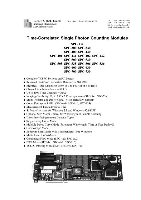
<strong>Time</strong>-<strong>Correlated</strong> <strong>Single</strong> <strong>Photon</strong> <strong>Counting</strong> <strong>Modules</strong><br />
SPC-134<br />
SPC-300 SPC-330<br />
SPC-400 SPC-430<br />
SPC-401 SPC-431 SPC-402 SPC-432<br />
SPC-500 SPC-530<br />
SPC-505 SPC-535 SPC-506 SPC-536<br />
SPC-600 SPC-630<br />
SPC-700 SPC-730<br />
♦ Complete TCSPC Systems on PC Boards<br />
♦ Reversed Start/Stop: Repetition Rates up to 200 MHz<br />
♦ Electrical <strong>Time</strong> Resolution down to 7 ps FWHM or 4 ps RMS<br />
♦ Channel Resolution down to 813 fs<br />
♦ Up to 4096 <strong>Time</strong> Channels / Curve<br />
♦ Imaging Capability: Up to 256 x 256 decay curves (SPC-5xx, SPC-7xx)<br />
♦ Multi Detector Capability: Up to 16 384 Detector Channels<br />
♦ Count Rate up to 8 MHz (SPC-4x0, SPC-6x0, SPC-134)<br />
♦ Measurement <strong>Time</strong>s down to 1 ms<br />
♦ Software Versions for Windows 3.1 and Windows 95/98/NT<br />
♦ Optional Step Motor Control for Wavelength or Sample Scanning<br />
♦ Direct Interfacing to most Detector Types<br />
♦ <strong>Single</strong> Decay Curve Mode<br />
♦ Multiple Decay Curve Mode (Parameter Wavelength, <strong>Time</strong> or User Defined)<br />
♦ Oscilloscope Mode<br />
♦ Spectrum Scan Mode with 8 Independent <strong>Time</strong> Windows<br />
♦ Multichannel X-Y-t-Mode<br />
♦ Continuous Flow Mode (SPC-4x0, SPC-6x0)<br />
♦ BIFL Mode (SPC-4x1, SPC-4x2, SPC-6x0)<br />
♦ TCSPC Imaging Modes (SPC-5x5/5x6, SPC-7x0)<br />
Tel. +49 / 30 / 787 56 32<br />
FAX +49 / 30 / 787 57 34<br />
http://www.becker-hickl.de<br />
email: info@becker-hickl.de
Table of Contents set 5 levels, user defined<br />
Introduction........................................................................................................................................................7<br />
General Features...........................................................................................................................................7<br />
Measurement Modes ....................................................................................................................................7<br />
Module Types...............................................................................................................................................8<br />
Accessories...................................................................................................................................................13<br />
<strong>Time</strong>-correlated single photon counting: General measurement principle.........................................................15<br />
Measurement System .........................................................................................................................................19<br />
General Principle..........................................................................................................................................19<br />
CFD and SYNC circuits .........................................................................................................................19<br />
TAC........................................................................................................................................................20<br />
ADC........................................................................................................................................................20<br />
Memory ..................................................................................................................................................20<br />
Memory Control .....................................................................................................................................20<br />
Memory Control in the Continuous Flow Mode.....................................................................................21<br />
Memory Control in the FIFO Mode........................................................................................................22<br />
Memory Control in the Scan SYNC Modes ...........................................................................................23<br />
Detailed Description of Building Blocks......................................................................................................25<br />
Constant Fraction Discriminator.............................................................................................................25<br />
SPC-x00 Versions.............................................................................................................................25<br />
SPC-x30 Versions.............................................................................................................................26<br />
Synchronisation Circuit ..........................................................................................................................27<br />
SPC-x00 Versions.............................................................................................................................27<br />
SPC-x30 Versions.............................................................................................................................28<br />
<strong>Time</strong>-to-Amplitude Converter ................................................................................................................29<br />
ADC with Error Correction ....................................................................................................................30<br />
Installation .........................................................................................................................................................33<br />
General Requirements ..................................................................................................................................33<br />
Software Installation - <strong>Single</strong> <strong>Modules</strong> ........................................................................................................33<br />
Software Installation - Multi SPC Systems ..................................................................................................33<br />
Software Update...........................................................................................................................................34<br />
Update from the Web .............................................................................................................................34<br />
Hardware Installation - <strong>Single</strong> SPC <strong>Modules</strong>...............................................................................................34<br />
Hardware Installation - Several SPC <strong>Modules</strong> .............................................................................................35<br />
Changing the Module Address (ISA <strong>Modules</strong>, SPC-3, -4, -5) .....................................................................35<br />
Using the SPC software without an SPC Module.........................................................................................36<br />
Operating the SPC Module ................................................................................................................................39<br />
Input Signal Requirements ...........................................................................................................................39<br />
Generating the Synchronisation Signal.........................................................................................................39<br />
Choosing and Connecting the Detector ........................................................................................................40<br />
MCP PMTs.............................................................................................................................................40<br />
Hamamatsu R5600 and Derivatives........................................................................................................40<br />
Conventional PMTs................................................................................................................................41<br />
Avalanche Photodiodes ..........................................................................................................................41<br />
Preamplifiers...........................................................................................................................................42<br />
Safety Recommendations........................................................................................................................42<br />
Optimising a TSPC System..........................................................................................................................43<br />
General Recommendations .....................................................................................................................43<br />
Configuring the CFD and SYNC Inputs .................................................................................................43<br />
Optimising the CFD and SYNC Parameters...........................................................................................44<br />
CFD Parameters................................................................................................................................44<br />
SYNC Parameters .............................................................................................................................45<br />
TAC Linearity.........................................................................................................................................45<br />
Optimising the Photomultiplier...............................................................................................................47<br />
<strong>Time</strong> Resolution................................................................................................................................47<br />
Voltage Divider...........................................................................................................................47<br />
Illuminated Area..........................................................................................................................48<br />
Signal-Dependent Background .........................................................................................................48<br />
Dark Count Rate ...............................................................................................................................49<br />
2
Checking the SER of PMTs.............................................................................................................. 49<br />
Optical System ....................................................................................................................................... 50<br />
Routing and Control Signals........................................................................................................................ 51<br />
SPC-300/330 and SPC-400/430............................................................................................................. 51<br />
SPC-500/530.......................................................................................................................................... 51<br />
SPC-503/535.......................................................................................................................................... 52<br />
SPC-506/536.......................................................................................................................................... 53<br />
SPC-600/630.......................................................................................................................................... 54<br />
SPC-700/730.......................................................................................................................................... 55<br />
SPC-134 ................................................................................................................................................. 58<br />
Getting Started............................................................................................................................................. 59<br />
Quick Startup ......................................................................................................................................... 59<br />
Startup for Beginners ............................................................................................................................. 59<br />
Applications ...................................................................................................................................................... 63<br />
Optical Oscilloscope.................................................................................................................................... 63<br />
Measurement of Luminescence Decay Curves ............................................................................................ 63<br />
Lock-in SPC................................................................................................................................................. 65<br />
Multiplexed TCSPC..................................................................................................................................... 66<br />
Multichannel Operation ............................................................................................................................... 67<br />
TCSPC Imaging........................................................................................................................................... 69<br />
The TCSPC Laser Scanning Microscope..................................................................................................... 71<br />
<strong>Single</strong> Molecule Detection........................................................................................................................... 72<br />
Measurements at low pulse repetition rates ................................................................................................. 73<br />
Non-Reversed Start-Stop ............................................................................................................................. 74<br />
Software ............................................................................................................................................................ 75<br />
Overview...................................................................................................................................................... 75<br />
Menu Bar ............................................................................................................................................... 76<br />
Curve Window ....................................................................................................................................... 76<br />
Count Rate Display ................................................................................................................................ 76<br />
Device State ........................................................................................................................................... 76<br />
System Parameter Settings ..................................................................................................................... 77<br />
Trace Statistics ....................................................................................................................................... 77<br />
Module Select (Multi SPC Software)..................................................................................................... 77<br />
Main............................................................................................................................................................. 79<br />
Load ....................................................................................................................................................... 79<br />
Data and Setup File Formats....................................................................................................... 79<br />
File Name / Select File................................................................................................................ 79<br />
File Info, Block Info ................................................................................................................... 79<br />
Load / Cancel.............................................................................................................................. 80<br />
Loading selected Parts of a Data File..........................................................................................80<br />
Loading Files from older Software Versions .............................................................................. 81<br />
Save (Non-FIFO Versions or Non-FIFO Modes only)........................................................................... 81<br />
File Format.................................................................................................................................. 81<br />
File Name.................................................................................................................................... 81<br />
File Info ...................................................................................................................................... 82<br />
Save / Cancel .............................................................................................................................. 82<br />
Selecting the data to be saved ..................................................................................................... 82<br />
Convert (Non-FIFO Versions or Non-FIFO Modes)............................................................................. 83<br />
Convert (FIFO Versions or FIFO Mode of the SPC-6).......................................................................... 84<br />
Print........................................................................................................................................................ 85<br />
Parameters ................................................................................................................................................... 87<br />
System Parameters ................................................................................................................................. 87<br />
Measurement Control ....................................................................................................................... 87<br />
Operation Modes .............................................................................................................................. 87<br />
<strong>Single</strong> (All SPC <strong>Modules</strong>)........................................................................................................... 88<br />
Oscilloscope (All SPC <strong>Modules</strong>) ............................................................................................... 88<br />
f(t,x,y) Mode (SPC-3x0, SPC-4x0, SPC-5x0, SPC-6x0, SPC-7x0)............................................ 89<br />
f(t,T) Mode (All SPC <strong>Modules</strong>).................................................................................................89<br />
f(t,EXT) Mode (All SPC <strong>Modules</strong>) ........................................................................................... 91<br />
fi(T) Mode (All SPC <strong>Modules</strong>).................................................................................................. 92<br />
3
fi(EXT) Mode (All SPC <strong>Modules</strong>).............................................................................................93<br />
Continuous Flow Mode (SPC-4x0, SPC-6x0 and SPC-134 only)...............................................94<br />
FIFO Mode (SPC-4x1/4x2 , SPC-6x0 and SPC-134only) ..........................................................95<br />
Scan Sync Out Mode (SPC-7x0 and SPC-5x5 only) ...................................................................96<br />
Scan Sync In Mode (SPC-7x0 and SPC-5x6 only)......................................................................96<br />
Scan XY Out Mode (SPC-700/730 only)....................................................................................98<br />
Control Parameters (Non-FIFO <strong>Modules</strong> or Non-FIFO Modes).......................................................98<br />
Control Parameters (FIFO <strong>Modules</strong> or FIFO Modes).......................................................................100<br />
Stepping Device (Non-FIFO Modes only)........................................................................................100<br />
Timing Control Parameters...............................................................................................................101<br />
CFD Parameters................................................................................................................................102<br />
Limit Low....................................................................................................................................102<br />
Limit High (SPC-x00 only) .........................................................................................................102<br />
ZC Level......................................................................................................................................102<br />
Hold (SPC-x00 only)...................................................................................................................102<br />
SYNC Parameters .............................................................................................................................102<br />
ZC Level......................................................................................................................................102<br />
Freq Div ......................................................................................................................................102<br />
Holdoff ........................................................................................................................................102<br />
Threshold (SPC-x30 only)...........................................................................................................103<br />
TAC Parameters................................................................................................................................103<br />
Range...........................................................................................................................................103<br />
Gain.............................................................................................................................................103<br />
Offset...........................................................................................................................................103<br />
Limit Low....................................................................................................................................103<br />
Limit High ...................................................................................................................................103<br />
<strong>Time</strong>/Ch.......................................................................................................................................103<br />
<strong>Time</strong>/div ......................................................................................................................................103<br />
Data Format ......................................................................................................................................104<br />
ADC Resolution (Non-FIFO Modes) ..........................................................................................104<br />
ADC Resolution (FIFO Modes) ..................................................................................................104<br />
Memory Offset (Non-FIFO Modes only) ....................................................................................104<br />
Dither Range ...............................................................................................................................105<br />
Count Increment (Non-FIFO Modes only)..................................................................................105<br />
FIFO Frame Length (SPC-6 in the FIFO Mode) .........................................................................105<br />
Page Control .....................................................................................................................................105<br />
Routing Channels X, Routing Channels Y ..................................................................................106<br />
Scan Pixels X, Scan Pixels Y (Scan Modes) ...............................................................................106<br />
Page (Non-FIFO Modes).............................................................................................................106<br />
Delay (Not for SPC-134).............................................................................................................106<br />
Memory Bank (SPC-400/430, SPC-600/630 and SPC-134 in NON-FIFO Modes)...................106<br />
More Parameters .........................................................................................................................106<br />
Parameter Management for Multi-SPC Configurations ....................................................................107<br />
Display Parameters .................................................................................................................................109<br />
General Display Parameters..............................................................................................................109<br />
2D Display Parameters......................................................................................................................110<br />
3D Display Parameters......................................................................................................................110<br />
3D Curve Mode Parameters ........................................................................................................111<br />
Colour-Intensity and OGL Mode Parameters..............................................................................112<br />
Trace Parameters ....................................................................................................................................113<br />
Trace Definitions ..............................................................................................................................113<br />
Block Info .........................................................................................................................................114<br />
Export of Trace Data.........................................................................................................................115<br />
Window Intervals....................................................................................................................................115<br />
<strong>Time</strong> Windows..................................................................................................................................115<br />
X Windows, Y Windows ..................................................................................................................116<br />
Auto Set Function .............................................................................................................................119<br />
Adjust Parameters...................................................................................................................................119<br />
Production Parameters ......................................................................................................................119<br />
Adjust Values....................................................................................................................................119<br />
4
Display Routines .................................................................................................................................... 121<br />
Display 2D........................................................................................................................................ 121<br />
Cursors........................................................................................................................................ 121<br />
Data Point ................................................................................................................................... 122<br />
Zoom Function............................................................................................................................ 122<br />
2D Data Processing..................................................................................................................... 122<br />
Curve Display 3D ............................................................................................................................. 123<br />
Cursors........................................................................................................................................ 123<br />
Data Point ................................................................................................................................... 124<br />
Zoom Function............................................................................................................................ 124<br />
3D Data Processing..................................................................................................................... 124<br />
Start, Interrupt, Stop .................................................................................................................................... 124<br />
Start........................................................................................................................................................ 124<br />
Interrupt.................................................................................................................................................. 125<br />
Stop ........................................................................................................................................................ 125<br />
Exit .............................................................................................................................................................. 125<br />
Data file structure .............................................................................................................................................. 126<br />
DOS Software and Windows Software SPC-300 V 1.6 and earlier............................................................. 126<br />
SPC Standard Software Version 2.0 to 6.9 .................................................................................................. 127<br />
File Header (binary) ............................................................................................................................... 127<br />
File Info.................................................................................................................................................. 127<br />
Setup ...................................................................................................................................................... 127<br />
Measurement Description Blocks........................................................................................................... 128<br />
Data Blocks............................................................................................................................................ 129<br />
SPC Standard Software Version 7.0 and later ............................................................................................. 130<br />
Multi-SPC Software Version 7.0 and later .................................................................................................. 130<br />
File Header (binary) ............................................................................................................................... 130<br />
File Info.................................................................................................................................................. 130<br />
Setup ...................................................................................................................................................... 131<br />
Measurement Description Blocks........................................................................................................... 131<br />
Data Blocks............................................................................................................................................ 132<br />
FIFO File Structure, Version 2.0 to 6.9 ....................................................................................................... 134<br />
Setup Files.............................................................................................................................................. 134<br />
File Header ....................................................................................................................................... 134<br />
Info ................................................................................................................................................... 134<br />
Setup Block ...................................................................................................................................... 135<br />
Measurement Data Files (SPC-401/431, SPC-6 FIFO 4096 Channels ) ................................................ 135<br />
Measurement Data Files (SPC-402/432, SPC-6 FIFO 256 Channels) ................................................... 136<br />
FIFO File Structure, Version 7.0 and later................................................................................................... 137<br />
Setup Files.............................................................................................................................................. 137<br />
File Header ....................................................................................................................................... 137<br />
Info ................................................................................................................................................... 137<br />
Setup Block ...................................................................................................................................... 138<br />
Measurement Data Files (SPC-401/431, SPC-6 FIFO 4096 Channels ) ................................................ 138<br />
Measurement Data Files (SPC-402/432, SPC-6 FIFO 256 Channels) ................................................... 139<br />
Measurement Data Files (SPC-134)....................................................................................................... 140<br />
Trouble Shooting............................................................................................................................................... 141<br />
How to Avoid Damage ................................................................................................................................ 141<br />
Testing the Module by the SPC Test Program............................................................................................. 142<br />
Test for Basic Function and for Differential Nonlinearity ........................................................................... 142<br />
Test for <strong>Time</strong> Resolution ............................................................................................................................. 143<br />
Frequently Encountered Problems ............................................................................................................... 143<br />
Assistance through bh .................................................................................................................................. 147<br />
Specification...................................................................................................................................................... 148<br />
SPC-300/330-10, SPC-300/330-12.............................................................................................................. 148<br />
SPC-400/430................................................................................................................................................ 149<br />
SPC-401/431, SPC-402/432 ........................................................................................................................ 150<br />
SPC-500/530................................................................................................................................................ 151<br />
SPC-505/535 and SPC-506/536 .................................................................................................................. 152<br />
SPC-600/630................................................................................................................................................ 153<br />
5
SPC-700/730 ................................................................................................................................................154<br />
SPC-134 .......................................................................................................................................................155<br />
Absolute Maximum Ratings (for all SPC modules) .....................................................................................156<br />
Index ..................................................................................................................................................................157<br />
6
Introduction<br />
General Features<br />
The SPC-300/330, SPC-400/430, SPC-500/530, SPC-600/630 and SPC-700/730 modules<br />
contain complete electronic systems for recording fast light signals by time-correlated single<br />
photon counting (TCSPC) on single PC boards. The Constant Fraction Discriminators<br />
(CFDs), the <strong>Time</strong>-to-Amplitude Converter (TAC), a fast Analog-to-Digital Converter (ADC)<br />
and the Multichannel Analyser (MCA) with the data memory and the associated control<br />
circuits are integrated on the board.<br />
The SPC-134 ‘TCSPC Power Package’ is a stack of four TCSPC modules. Each module is a<br />
complete TCSPC system and contains its own CFDs, TAC, ADC and MCA.<br />
All functions of the SPC modules are controlled by a common ‘SPC Standard Software’. The<br />
software provides functions such as set-up of measurement parameters, 2-dimensional and 3dimensional<br />
display of measurement results, mathematical operations, selection of subsets<br />
from 4 dimensional data sets, loading and saving of results and system parameters, control of<br />
the measurement in the selected operation mode, etc. With an optional step motor controller<br />
the software is able to control a monochromator or to scan a sample. The SPC Standard<br />
Software runs under Windows 3.1, Windows 95/98 and Windows NT.<br />
The SPC-3.. through SPC-7.. modules are available in two versions. These 00 and 30 versions<br />
differ in the input voltage range and the time resolution. The 00 modules work with input<br />
signals from ±10 mV to ±80 mV and can therefore be used without preamplifiers in most<br />
cases. The electrical time resolution of the SPC-x00 is 10 ps FWHM or 5 ps RMS typically.<br />
The SPC-x30 modules have an input voltage range from -50 mV to -1 V and an electrical time<br />
resolution of 8 ps FWHM or 4 ps RMS.<br />
All SPC systems are designed to work in the reversed start-stop mode. This enables operation<br />
at the full repetition rate of mode-locked cw lasers. Effective count rates of more than 4*106 photons/s can be achieved (SPC-4x0, SPC-6x0). Therefore results are obtained with data<br />
acquisition times down to 1 ms. The systems can be used to investigate transient phenomena<br />
or other variable effects in the sample. Furthermore, the SPC modules can be used as high<br />
resolution optical oscilloscopes with a sensitivity down to the single photon level.<br />
The SPC-300 through SPC-730 modules have built in multichannel and multidetector<br />
capabilities. In the device memory space is provided for several waveforms, and the<br />
destination of each individual photon is controlled by an external signal. In conjunction with a<br />
fast scanning device, time resolved images are obtained with up to 256 x 256 pixels<br />
containing a complete waveform each. Furthermore, several detectors can be used with one<br />
TCSPC module. This technique makes use of the fact that a simultaneous detection of several<br />
photons in different detectors is very unlikely. Therefore, the output pulses of all detectors are<br />
processed in one TCSPC channel and an external ‘Routing’ device determines in which<br />
detector a particular photon was detected. The routing information is used to store the photons<br />
from different detectors in different memory blocks.<br />
A digital lock-in technique is provided to suppress scattered light and detector background<br />
pulses. In conjunction with fast optical scanning devices or flip-mirror arrangements<br />
multiplexing into 128 waveform channels is achieved.<br />
Measurement Modes<br />
The SPC systems provide the following basic measurement modes:<br />
uneven page<br />
7
In the '<strong>Single</strong>' mode the intensity versus time (usually a fluorescence decay curve) is<br />
measured. In the 'Oscilloscope' mode a repetitive measurement is performed and the results<br />
are displayed in short intervals. Multichannel operation is possible in both modes with up to<br />
eight detector channels displayed simultaneously.<br />
In the 'f(t,T)' mode the measurement is repeated in specified time intervals. The results<br />
represent the change of the measured waveform (decay curve) with the time. In the 'f(t,EXT)'<br />
mode an external parameter is controlled via the optional step motor controller. The results<br />
represent the change of the waveform as a function of the external parameter (usually<br />
wavelength or sample displacement).<br />
In the 'fi(ext)' and fi(T)' modes time resolved spectra are recorded. Up to 8 time independent<br />
time windows can be selected on the measured waveforms, and the intensities within these<br />
windows are displayed as a function of time or an externally variable parameter.<br />
The 'f(t,x,y)' mode is used for multichannel measurements with detector arrays. Up to 128<br />
decay curves (16384 for the SPC-5 and -7) can be recorded simultaneously and displayed as<br />
f(t,x), f(t,y) or f(x,y).<br />
The 'Continuous Flow' mode is available in the SPC-400/430, the SPC-600/630 and in the<br />
SPC-134 only. The 'Continuous Flow' mode is targeted at single molecule detection in a<br />
continuous flow setup and other applications which require a large number of curves to be<br />
recorded in defined (or short) time intervals without time gaps between subsequent<br />
recordings. Unlike f(t,T), the ‘Continuous Flow’ mode is strictly hardware controlled and thus<br />
provides an extremely accurate recording sequence.<br />
The 'FIFO' mode is available in the SPC-4x1/4x2, the SPC-600/630 and the SPC-134. This<br />
mode is used for single molecule investigations by the ‘BIFL’ method. For each photon the<br />
time within the laser pulse sequence and the time from the start of the experiment is stored.<br />
The memory is configured as a FIFO (First In First Out) buffer. During the measurement, the<br />
FIFO is continuously read by the device software and the results are stored to the hard disk of<br />
the computer.<br />
The ‘Scan’ and ‘TV’ modes are used for image recording with the SPC-505/535/506/536 and<br />
in the SPC-700/730 modules. In conjunction with a laser scanning microscope or another<br />
scanning device, these modes acquire images with up to 65535 pixels containing a complete<br />
waveform each.<br />
Module Types<br />
SPC-300/330<br />
The SPC-300/330 is the TCSPC module for basic applications. It comes in two versions. The<br />
SPC-300/330-10 have up to 128 detector channels and a resolution of 1024 points per curve,<br />
the SPC-300/330-12 have up to 32 detector channels and a resolution of 4096 points per<br />
curve. Although the SPC-300/330 was the first of all BH TCSPC modules it is far from being<br />
obsolete. It has continuously been upgraded with the development of newer modules and<br />
contains the same CFD, SYNC, TAC and ADC modules as the latest SPC-6 and SPC-7 PCI<br />
bus modules.<br />
SPC-400/430<br />
The SPC-400/430 modules differ from the SPC300/330 in that they use a dual memory<br />
structure for simultaneous measurement and data readout. Furthermore, the exceptionally low<br />
dead time of the SPC-4 modules allows high count rates. This makes the SPC-400/430 an<br />
excellent choice for all applications which require maximum data throughput. A ‘Continuous<br />
8
Flow’ mode is implemented for single molecule detection in a continuos flow arrangement. It<br />
continuously records decay curves with short collection times and without time gaps between<br />
subsequent recordings and stores the results to the hard disk.<br />
Of course the SPC-400/430 can also be used for the traditional applications. Recording of<br />
fluorescence decay curves, time-resolved fluorescence spectra, multi-detector measurements<br />
etc. can be done in the same way as with the SPC-300/330.<br />
SPC-401/431, SPC-402/432<br />
The SPC-401/431 and SPC-402/432 are designed for single molecule detection by the BIFL<br />
method. They employ a fast FIFO memory to store the time within the excitation pulse<br />
sequence, the time from the start of the experiment and the detector channel for each detected<br />
photon. During the measurement, the FIFO is continuously read by the device software and<br />
the results are stored to the hard disk of the computer. Due to an extremely fast signal<br />
processing circuitry and a large FIFO size burst count rates of more than 4*106 photons/s can<br />
be recorded for more than 10 ms.<br />
The SPC-401/431 and SPC-402/432 modules differ in the data format in which the photon<br />
information is stored. The SPC-401/431 data contain 4096 time channels and 128 detector<br />
channels thus providing a minimum time channel width of 813 fs and a FIFO size of 64k<br />
photons. The SPC-402/432 uses a reduced data format containing 256 time channels and 8<br />
detector channels only. This gives a minimum time channel width of 13 ps while increasing<br />
the FIFO size to 128k photons.<br />
SPC-500/530<br />
The SPC-500/530 modules have extremely large memories and are targeted at fast scanning<br />
and imaging applications. Up to 16384 decay curves can be measured simultaneously. A<br />
14 bit routing signal is used to select the curve into which a detected photon is stored. In<br />
scanning applications this signal must be provided by the scanning device.<br />
The SPC-500/530 work also for the traditional applications. Recording of fluorescence decay<br />
curves, time-resolved fluorescence spectra etc. can be done in the same way as with the SPC-<br />
300/330 and in the SPC-400/430. However, the maximum count rate is lower due to the<br />
higher dead time.<br />
SPC-505/535<br />
These modules are special versions of the SPC-500/530. They are designed for use with a<br />
scanning device that is controlled by the SPC module. The modules acquire images with up to<br />
16384 pixels containing a complete waveform each. The SPC-505/535 internally steps<br />
through the pixels of the recorded image while delivering signals to control an external<br />
scanning device.<br />
The SPC-505/535 work also for the traditional applications. Recording of fluorescence decay<br />
curves, time-resolved fluorescence spectra etc. can be done in the same way as with the SPC-<br />
300/330 and in the SPC-400/430. However, multi-detector measurements are not possible<br />
with the SPC-505/535 and the maximum count rate is lower due to the higher dead time.<br />
SPC-506/536<br />
The SPC-506/536 accepts synchronisation signals from ultra-fast video-compatible scanners<br />
from which the stepping through the pixels of the image is derived. As the other SPC-5<br />
modules, the SPC-506/536 acquire images with up to 16384 pixels containing a complete<br />
waveform each.<br />
9
The SPC-505/535 work also for the traditional applications. Recording of fluorescence decay<br />
curves, time-resolved fluorescence spectra etc. can be done in the same way as with the SPC-<br />
300/330 and in the SPC-400/430. However, multi-detector measurements are not possible<br />
with the SPC-505/535 and the maximum count rate is lower due to the higher dead time.<br />
SPC-600/630 - the TCSPC General Solution<br />
The SPC-600/630 PCI bus modules combine the features of the SPC-400/430, SPC-401/431<br />
and the SPC-402/432 modules. They use a dual memory structure for simultaneous<br />
measurement and data readout. The exceptionally low dead time of the SPC-6 modules allows<br />
high count rates. This makes the SPC-600/630 an excellent choice for all applications which<br />
require maximum data throughput. A ‘Continuous Flow’ mode is implemented for single<br />
molecule detection in a continuos flow arrangement. It continuously records decay curves with<br />
short collection times and without time gaps between subsequent recordings and stores the<br />
results to the hard disk.<br />
Furthermore, the SPC-6 modules can be configured for single molecule detection by the BIFL<br />
method. In this mode the device memory is configured as a fast FIFO memory to store the<br />
time within the excitation pulse sequence, the time from the start of the experiment and the<br />
detector channel for each individual photon. During the measurement, the FIFO is<br />
continuously read by the device software and the results are stored to the hard disk of the<br />
computer. Due to an extremely fast signal processing circuitry and a large FIFO size burst<br />
count rates of more than 4*106 photons/s can be recorded for more than 10 ms.<br />
Thus, the SPC-600/630 modules are an excellent choice for the complete range from the<br />
traditional fluorescence lifetime experiments to single molecule fluorescence lifetime<br />
investigations.<br />
SPC-700/730 - the TCSPC Imaging Solution<br />
The SPC-700/730 PCI bus modules combine the features of the SPC-500/530, SPC-505/535<br />
and the SPC-506/536 modules. Therefore, the SPC-700/730 is the solution for all TCSPC<br />
scanning and imaging applications.<br />
Due to their flexible scanning interface, the SPC-7 modules can be coupled to almost any<br />
scanning device. The modules can be synchronised by the frame/line synchronisation pulses or<br />
by X/Y signals from free running scanners such as confocal laser scanning microscopes or<br />
ultra-fast video-compatible scanners. Furthermore, the SPC-7 modules can actively control a<br />
scanning device by sending appropriate synchronisation pulses or X/Y signals. The maximum<br />
scanning area is 128 x 128 pixels for the X/Y control modes and 256 x 256 pixels for the<br />
modes using synchronisation pulses.<br />
The SPC-700/730 work also for the traditional applications. Fluorescence decay curves, timeresolved<br />
fluorescence spectra etc. can be recorded in the same way as with the SPC-300/330<br />
and in the SPC-400/430.<br />
SPC-134 - The TCSPC Power Package<br />
The SPC-134 is a stack of four completely independent TCSPC modules. Due to space, power<br />
supply and price constraints the SPC-134 channels have reduced routing capabilities and are<br />
available only in the 3x version, i.e. for negative input signals. However, no compromises<br />
have been made for the essential parameters as count rate, time resolution, or differential<br />
nonlinearity. The SPC-134 requires the ‘Multi SPC Software’ and works in the <strong>Single</strong>,<br />
Oscilloscope, f(t,T), f(t, ext), fi(T), fi(ext) and in the Continuous Flow and FIFO mode.<br />
10
With its four channels and 32 MHz overall count rate the SPC-134 is an extremely powerful<br />
solution for all applications which require maximum data throughput. Although the SPC-134<br />
can be used for traditional fluorescence experiments the typical applications are for optical<br />
tomography, stopped flow experiments and single molecule detection.<br />
A comparison of the different SPC versions is given in the table on the next page.<br />
11
SPC-300 SPC-330 SPC-400 SPC-430 SPC-401 SPC-431 SPC-500 SPC-530 SPC-505 SPC-535 SPC-600 SPC-630 SPC-700 SPC-730 SPC-134<br />
-10 -12 -10 -12 SPC-402 SPC-432 SPC-506 SPC-536<br />
TCSPC Channels 1 1 1 1 1 1 1 1 1 1 1 1 1 1 4<br />
Points /Curve 1024 4096 1024 4096 64, 256, 1024, 4096 64, 256, 1024, 4096 64, 256, 1024, 4096 64, 256, 1024, 4096 64, 256, 1024, 4096 64, 256, 1024, 4096<br />
Curves in Memory 128 32 128 32 32..128 up to 16384 up to 16384 32..128 up to 65536 32..128<br />
Input Voltage 10..80 mV 50mV..2V 10..80 mV 50mV..2V 10..80 mV 50mV..2V 10..80 mV 50mV..2V 10..80 mV 50mV..2V 10..80 mV 50mV..2V 10..80 mV 50mV..2V 50mV..2V<br />
<strong>Time</strong> Resol. (el., FWHM) 11 ps 6 ps 11 ps 7 ps 11 ps 7 ps 11 ps 7 ps 11 ps 7 ps 11 ps 7 ps 11 ps 7 ps 7 ps<br />
<strong>Time</strong> Resol. (MCP, FWHM) 30 ps 25 ps 30 ps 25 ps 30 ps 25 ps 30 ps 25 ps 30 ps 25 ps 30 ps 25 ps 30 ps 25 ps 25 ps<br />
Dead <strong>Time</strong> 200 ns 200 ns 125 ns 125 ns 125 ns 125 ns 330ns 330ns 330ns 330ns 125 ns 125 ns 330ns 330ns 125ns<br />
Count Rate Limit 5 MHz 5 MHz 8 MHz 8 MHz 8 MHz 8 MHz 3 MHz 3 MHz 3 MHz 3 MHz 8 MHz 8 MHz 5.5 MHz 5.5 MHz 8 MHz per Channel<br />
Memory (MCA) single single dual dual FIFO FIFO single single single single dual/FIFO dual/FIFO single single dual<br />
Multi-Detector Operation yes yes yes yes yes yes yes yes no no yes yes yes yes no<br />
Readout during Measurement no no yes yes yes yes no no no no yes yes no no yes<br />
Count Rate Display yes yes yes yes yes yes yes yes yes yes yes yes yes yes yes<br />
Sync Rate Display no no no yes no yes no yes no yes no yes no yes yes<br />
Dead <strong>Time</strong> Compensation yes yes on/off on/off on/off on/off on/off on/off on/off on/off on/off on/off on/off on/off on/off<br />
‘Start Measurement’ Trigger no no no no no no no no no no yes yes yes yes yes<br />
PC Bus Interface<br />
Application for<br />
ISA ISA ISA ISA ISA ISA ISA ISA ISA ISA PCI PCI PCI PCI PCI<br />
Optical Oscilloscope X X X X X X X X X X X X x<br />
Fluorescence Decay X X X X X X X X X X X X x<br />
Fluorescence Spectra X X X X X X X X X X X X x<br />
<strong>Photon</strong> Correlation X X x x X x X<br />
<strong>Single</strong> Molecule (CFD) X X X X X<br />
<strong>Single</strong> Molecule (BIFL) X X X X X<br />
Opt. Tomography x x x x X X X X x x X X X<br />
Lifetime Imaging X X X X X X<br />
Fast Image Scanning x x X X X X<br />
X = recommended<br />
x = applicable, but other versions give better performance or lower cost
Accessories<br />
Preamplifiers<br />
If the SPC-x30 modules are used with PMTs and MCPs preamplifiers are recommended. The<br />
SPC-x00 can be used without preamplifiers. However, to achieve optimum resolution with<br />
MCPs and to extend the lifetime of these detectors preamplifiers should be used also for the<br />
SPC-x00 modules. For safe operation of MCPs and PMTs the HFAC-26 amplifier (26 dB, 1.6<br />
GHz) with current sensing is available. This amplifier indicates overload conditions in the<br />
detector by a LED and by a TTL signal. For multidetector measurements the HFAM-26 with<br />
eight amplifier channels is available. Other amplifiers are the ACA-2 and ACA-4 devices with<br />
gains from 10 dB to 40 dB and a bandwidth up to 2 GHz.<br />
Detectors<br />
A wide variety of PMT and MCP detectors can be delivered with the SPC modules. This<br />
includes also cooling devices and high voltage power supplies. As a simple and rugged<br />
solution the PMH-100 detector head is available. This device contains a fast, small PMT, the<br />
high voltage generator and a preamplifier altogether in a 32x38x92mm housing. The<br />
PMH-100 is powered directly from the SPC module - no high voltage power supply is<br />
required. For 16-channel measurements the PML-16 detector head is available.<br />
Diode Lasers<br />
The BHL-150 pulsed diode laser modules offer low cost, short pulse width and high repetition<br />
rate. They can be used for fluorescence excitation from 635 nm to 780 nm and for testing<br />
purposes.<br />
Reference Photodiodes<br />
To generate the synchronisation signal for the SPC from a laser pulse sequence fast<br />
photodiode modules are available. The PHD-400 and PDM-400 use fast PIN photodiodes. If<br />
high sensitivity is required the APM-400 avalanche photodiode modules are recommended.<br />
All photodiode modules are powered directly from the SPC card.<br />
Step Motor Controller<br />
For driving a monochromator or scanning a sample the Step Motor Controller STP-240 is<br />
available. The STP-240 drives up to two unipolar 4 phase motors with up to 1 A phase<br />
current. The electrical and mechanical drive parameters are set via a configuration file. The<br />
control software for the STP-240 is included in the SPC software.<br />
Routing devices<br />
The HRT-41 and HRT-81 routers are used to connect up to four (eight) individual PMTs or<br />
MCPs to one bh SPC module. To connect up to eight APD modules the HRT-82 is available.<br />
With the HRT devices, all detector channels work simultaneously and the detected photons<br />
are ‘routed’ into individual memory blocks (see 'Multichannel Measurements' and individual<br />
descriptions and data sheets).<br />
Adapters<br />
To connect signals from different sources to the SPC modules a wide variety of adapters are<br />
available. This includes attenuators and inverting transformers for TTL signals (e.g. from<br />
SPCM-AQR avalanche photodiode modules).
uneven page<br />
<strong>Time</strong>-correlated single photon counting: General measurement<br />
principle<br />
<strong>Time</strong>-<strong>Correlated</strong> <strong>Single</strong> <strong>Photon</strong> <strong>Counting</strong> is based on the detection of single photons of a<br />
periodical light signal, the measurement of the detection times of the individual photons and<br />
the reconstruction of the waveform from the individual time measurements.<br />
The method makes use of the fact that for low level, high repetition rate signals the light<br />
intensity is usually so low that the probability to detect one photon in one signal period is<br />
much less than one. Therefore, the detection of several photons can be neglected and the<br />
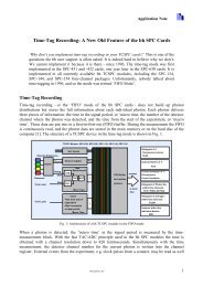
principle shown in the figure below can be used.<br />
The detector signal consists of a train of<br />
randomly distributed pulses due to the<br />
detection of the individual photons. There<br />
are many signal periods without photons,<br />
Original Waveform<br />
other signal periods contain one photon<br />
pulse. Periods with more than one photons<br />
Detector<br />
Signal:<br />
<strong>Time</strong><br />
are very rare.<br />
Period 1<br />
Period 2<br />
When a photon is detected, the time of the Period 3<br />
corresponding detector pulse is measured.<br />
The events are collected in a memory by<br />
Period 4<br />
Period 5<br />
Period 6<br />
adding a ‘1’ in a memory location with an Period 7<br />
address proportional to the detection time.<br />
Period 8<br />
After many photons, in the memory the<br />
histogram of the detection times, i.e. the<br />
Period 9<br />
Period 10<br />
waveform of the optical pulse builds up.<br />
Period N<br />
Although this principle looks complicated<br />
at first glance, it is very efficient and<br />
accurate for the following reasons:<br />
Result<br />
after many<br />
<strong>Photon</strong>s<br />
The accuracy of the time measurement is<br />
not limited by the width of the detector<br />
pulse. Thus, the time resolution is much<br />
better then with the same detector used in front of an oscilloscope or another analog signal<br />
acquisition device. Furthermore, all detected photons contribute to the result of the<br />
measurement. There is no loss due to ‘gating’ as in ‘Boxcar’ devices or gated image<br />
intensified CCDs.<br />
Depending on the desired accuracy, the light intensity must be not higher than to detect 0.1 to<br />
0.01 photons per signal period. Modern laser light sources deliver pulses with repetition rates<br />
of 50..100MHz. For these light sources, the count rate constraint is satisfied even at count<br />
rates of several 106 Fig. 1: TCSPC Measurement Principle<br />
photons per second. Such count rates already cause overload in many<br />
detectors. Consequently the intensity limitation of the SPC method does not cause problems in<br />
conjunction with high repetition rate laser light sources.<br />
Sensitivity<br />
The sensitivity of the SPC method is limited mainly by the dark count rate of the detector.<br />
Defining the sensitivity as the intensity at which the signal is equal to the noise of the dark<br />
signal the following equation applies:<br />
15
(Rd * N/T) 1/2<br />
S = ----------------<br />
Q<br />
(Rd = dark count rate, N = number of time channels, Q = quantum efficiency of the detector,<br />
T = overall measurement time)<br />
Typical values (PMT with multialkali cathode without cooling) are Rd=300s-1, N=256, Q=0.1<br />
and T=100s. This yields a sensitivity of S=280 photons/second. This value is by a factor of<br />
1015 smaller than the intensity of a typical laser (1018 photons/second). Thus, when a sample<br />
is excited by the laser and the emitted light is measured, the emission is still detectable for a<br />
conversion efficiency of 10 -15. <strong>Time</strong> resolution<br />
The SPC method differs from methods with analog signal processing in that the time<br />
resolution is not limited by the width of the detector impulse response. For the SPC method<br />
the timing accuracy in the detection channel is essential only. This accuracy is determined by<br />
the transit time spread of the single photon pulses in the detector and the trigger accuracy in<br />
the electronic system. The timing accuracy can be up to 10 times better than the half width of<br />
the detector impulse response. Some typical values for different detector types are given<br />
below.<br />
conventional photomultipliers<br />
standard types 0.6 ... 1 ns<br />
high speed (XP2020)<br />
Hamamatsu TO8 photomultipliers<br />
0.35 ns<br />
R5600, R5783<br />
micro channel plate photomultipliers<br />
140 ... 220 ps<br />
Hamamatsu R3809 25 ... 30 ps<br />
avalanche photodiodes 60 ... 500 ps<br />
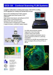
Accuracy<br />
The accuracy of the measurement is given by the<br />
standard deviation of the number of collected<br />
photons in a particular time channel. For a given<br />
number of photons N the signal-to-noise ratio is<br />
SNR = N 1/2 . If the light intensity is not too high,<br />
nearly all detected photons contribute to the<br />
result. Therefore, the SPC yields the maximal<br />
signal-to-noise ratio for a given intensity and<br />
measurement time. Furthermore, for the SPC<br />
method noise due leakage currents, gain<br />
instabilities, and the stochastic gain mechanism<br />
of the detector does not appear in the result. This<br />
yields an additional SNR improvement<br />
compared to analog signal processing methods.<br />
A laser pulse recorded with 30 ps fwhm<br />
Fluorescence decay curves, excitation with Ar+<br />
laser<br />
16
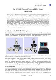
Recording Speed<br />
The TCSPC method is often thought to suffer<br />
from slow recording speed and long<br />
measurement times. This ill reputation<br />
comes from traditional TCSPC devices built<br />
up from nuclear instrumentation modules<br />
which had a maximum count rate of some<br />
10 4 photons per second. State-of-the-art<br />
TCSPC devices from <strong>Becker</strong> & <strong>Hickl</strong> achieve<br />
count rates of some 10 6 photons per seconds.<br />
Thus, 1000 photons can be collected in less<br />
than 1 ms, and the devices can be used for<br />
high speed applications such as the detection<br />
of single molecules flowing through a<br />
capillary, fast image scanning, for the<br />
investigation of unstable samples or simply as<br />
optical oscilloscopes.<br />
Multichannel and Multidetector<br />
Capability<br />
<strong>Becker</strong> & <strong>Hickl</strong> from the beginning have<br />
introduced multichannel and multidetector<br />
capabilities into their TCSPC modules. In the<br />
device memory space is provided for several<br />
waveforms, and the destination of each<br />
individual photon is controlled by an external<br />
signal. In conjunction with a fast scanning<br />
device, time resolved images are obtained<br />
with up to 256 x 256 pixels containing a<br />
complete waveform each.<br />
Furthermore, several detectors can be used<br />
with one TCSPC modules. This technique<br />
makes use of the fact that a simultaneous<br />
detection of several photons in different<br />
detectors is very unlikely. Therefore, the<br />
output pulses of the detectors are processed<br />
by only one TCSPC channel and an external<br />
‘Routing’ device determines in which<br />
detector a particular photon was detected.<br />
This information is used to route the photons<br />
into different memory blocks containing the<br />
waveforms for the individual detectors.<br />
Fluorescence decay signals from single molecules<br />
running through a capillary. Collection time 1 ms per<br />
curve.<br />
A 128 x 128 pixel scan containing 16384 waveforms<br />
16 signals measured simultaneously with a 16 channel<br />
PMT<br />
17
Measurement System<br />
General Principle<br />
The general principle of the bh TCSPC modules is shown in the figure below.<br />
ADD<br />
CNT<br />
Routing<br />
PMT<br />
SYNC<br />
CFD<br />
SYNC<br />
start<br />
stop<br />
CFD and SYNC circuits<br />
DEL<br />
TAC<br />
res<br />
WD<br />
LATCH<br />
PGA ADC<br />
ADD<br />
CNT<br />
Routing<br />
ASC<br />
MEM MEM<br />
(SPC-4x0,<br />
SPC-6x0)<br />
The single-photon pulses from the photon detector are fed to the input 'PMT'.<br />
Due to the stochastic gain mechanism in the detector these pulses have a<br />
considerable amplitude jitter (figure right). The constant fraction<br />
discriminator, CFD has to deliver an output pulse that is correlated as exactly<br />
as possible with the temporal location of the detector pulse. This is achieved<br />
by triggering on the zero cross point of the sum of the input pulse and the<br />
delayed and inverted input pulse (figure below, right).<br />
Since the temporal position of the crossover point is independent of the pulse<br />
amplitude, this timing method minimises the time jitter due to the amplitude<br />
jitter of the detector pulses. Furthermore, the CFD contains<br />
a window discriminator that rejects input pulses smaller than<br />
the discriminator threshold (SPC-x3x) or outside the selected<br />
amplitude window (SPC-x0x). The threshold or the<br />
amplitude window are adjusted to reject noise from the<br />
environment, noise from preamplifiers or small background<br />
pulses of the detector.<br />
The input signal SYNC is derived from the pulses of the<br />
light source and is used to synchronise the time measurement<br />
with the light pulses. The SYNC signal is received by the<br />
SYNC circuit which, as the CFD, has a fraction trigger<br />
characteristics to reduce the influence of amplitude<br />
fluctuations. Controlled by the software, the internal SYNC<br />
frequency can be divided by a factor of 2...16. In this case<br />
Input Pulse<br />
Delayed and<br />
Inverted Pulse<br />
uneven page<br />
<strong>Single</strong> <strong>Photon</strong><br />
Pulses of a PMT<br />
Zero Cross Point<br />
Independent of Amplitude<br />
Zero Cross Triggering<br />
several signal periods are displayed in the result. At very high pulse repetition rates the<br />
frequency divider may be used to reduce the internal synchronisation frequency.<br />
19
TAC<br />
The time-to-amplitude converter, TAC, is used to determine the temporal position of a<br />
detected photon within the SYNC pulse train. When the TAC is started by a pulse at the start<br />
input, it generates a linear ramp voltage until a stop pulse appears at the stop input. Thus the<br />
TAC generates an output voltage depending linearly on the temporal position of the photon.<br />
The time measurement is done from the photon to the next SYNC pulse. This 'reversed startstop'<br />
method is the key to process high photon count rates at high pulse repetition rates. It<br />
reduces the speed requirements to the TAC because its working cycle (start-stop-reset) has to<br />
be performed with the photon detection rate instead of the considerably higher pulse repetition<br />
rate.<br />
The TAC output voltage is fed to the programmable gain amplifier, PGA. The PGA is used to<br />
stretch a selectable part of the TAC characteristic over the complete measurement time<br />
window. To increase the effective count rate at high PGA gains, the output voltage of the<br />
PGA is checked by the window discriminator WD which rejects the processing of events<br />
outside the time window of interest.<br />
ADC<br />
The analog-digital converter, ADC, converts the amplified TAC signal into the address of the<br />
memory, MEM. The ADC must work with an extremely high accuracy. It has to resolve the<br />
TAC signal into 4096 time channels, and the width of the particular channels must be equal<br />
within 1..2%. This requires a 'no missing code' accuracy of more than 18 bits. This accuracy<br />
cannot be achieved with fast ADCs which are, however, required to achieve a high count rate.<br />
In the bh SPC modules the problem is solved with a fast flash ADC of 12 bit 'no missing code'<br />
accuracy in conjunction with a proprietary error correction method. The error correction is<br />
described in the section 'ADC with Error Correction'.<br />
Memory<br />
The address delivered by the ADC is proportional to the temporal position of the photon<br />
within the SYNC pulse train. Together with some external ‘Routing’ bits it controls the<br />
address of the device memory MEM. When a photon is detected, the contents of the addressed<br />
memory location is increased by a fixed increment. This is done by the add/subtract circuit,<br />
ASC. The ASC is able to add or subtract a selectable number from 1 to 255. Values >1 are<br />
used to get full scale recordings in short collection times (e.g. in the oscilloscope mode).<br />
Furthermore, the circuit delivers an overflow signal when the memory contents of the<br />
addressed memory location has reached its maximum value. In this moment the measurement<br />
can be stopped automatically.<br />
In the SPC-400/430, the SPC-600/630 and the SPC-134 modules a ‘dual memory’ structure is<br />
implemented. For sequential curve recording, the dual memory structure allows to continue<br />
the measurement in the second memory bank when the data from first bank is read and vice<br />
versa. Thus, an unlimited sequential recording without gaps between subsequent curves is<br />
achieved.<br />
Memory Control<br />
Multidetector operation is achieved by controlling the higher memory address bits by the<br />
external ‘Routing’ signal. The routing bits (6 in the SPC-3/12, 7 in the SPC-3/10 and the<br />
SPC-4 and -6, 14 in the SPC-5, and -7) control the higher address bits of the memory. Thus,<br />
by the routing signal the recorded photons are ‘routed’ into different part of the memory. Each<br />
selected memory part represents an individual curve (waveform). Corresponding to the<br />
20
number of routing bits, the maximum number of curves is 32 for the SPC-3x0-12, 128 for the<br />
SPC-3x0-10 and the SPC-4x0 and -6x0 and 16384 for the SPC-5 and -7.<br />
Furthermore, the higher memory address can be controlled internally. In this case the number<br />
of curves can be much higher, i.e. 4096 for the SPC-6 and 65536 for the SPC-7.<br />
By the implemented memory control new powerful measurement modes become possible<br />
which are beyond the reach of conventional TCSPC devices:<br />
Several light signals can be measured quasi-simultaneously with one detector by multiplexing<br />
the light signals and controlling the destination curve by the routing signals (see also<br />
‘Multiplexed SPC’). With optical scanners (e.g. a laser scanning microscope) images can be<br />
recorded with up to 256 x 256 pixels (SPC-7) containing a complete decay curve each.<br />
Simultaneous multichannel operation with several detectors is accomplished by combining the<br />
photon pulses from all detectors into one common timing pulse and providing a routing signal<br />
which directs the photons from the individual detectors into different memory blocks (see also<br />
'Multichannel Measurements'). Routing devices for individual detectors are available for 4 and<br />
8 detector channels (HRT-4 and HRT-8). Complete detector heads are available with 16<br />
channels in a linear arrangement.<br />
If external parameters are changed during the measurement (temperature, oxygen pressure,<br />
location on the sample) and an appropriate routing signal is provided, a sequence of decay<br />
curves for different parameter values can be recorded. The routing capability can even be used<br />
to record signals from intrinsically variable objects. If a routing signal describing the state of<br />
the object is can be provided, the photons from the object are routed to different curves<br />
depending on the state of the object. The result of the measurement are several decay<br />
functions recorded in different states of the object.<br />
In all SPC modules the destination curve of the recorded photons can also be controlled by<br />
software. Controlled by the on-board timers, a sequence of subsequent decay curves can be<br />
recorded. In the SPC-134, SPC-6 and SPC-7 the start of a sequence can be triggered, and<br />
several sequences can be accumulated. This allows to record transient phenomena in the decay<br />
curves down the ms time scale and below.<br />
CNT and ADD Control<br />
Additional control over the measurement is given by the signals CNT and ADD. CNT is a<br />
‘Count Enable’ signal, i.e. a photon is stored only if CNT is ‘1’ in the moment of its<br />
detection. The CNT signal is used to suppress photons for which no valid routing information<br />
is provided or to confine the recording to externally controlled time intervals.<br />
The ADD signal controls whether a photon is added or subtracted. This enables the SPC to be<br />
combined with a digital lock-in technique. By using an optical system with light choppers or<br />
rotating sector mirrors background or the scattered light signals can be suppressed (see also<br />
‘Lock-in SPC).<br />
All external control signals are read by the latch register LATCH. The signals are latched at an<br />
adjustable delay time after the start pulse. By adjusting this delay it can be assured that every<br />
photon be processed with the corresponding state of the control signals.<br />
Memory Control in the Continuous Flow Mode<br />
In the SPC-400/430, the SPC-600/630 and the SPC-134 modules a ‘Continuous Flow’ mode<br />
is implemented which is used to record a virtually unlimited number of decay curves. The<br />
Continuous Flow Mode makes use of the two independent memory banks which are<br />
implemented in the SPC-4, SPC-6 and SPC-134 modules. As usual, the decay curves are<br />
21
measured in intervals of ‘Collection <strong>Time</strong>’. However, the measurement is repeated while the<br />
measurement system automatically switches through all memory blocks of both memory<br />
banks. While the measurement is running in one memory bank, the results of the other bank<br />
are read and stored to the hard disk. Thus, a virtually unlimited number of decay curves can be<br />
recorded without time gaps between subsequent curves.<br />
CFD<br />
SYNC<br />
TAC ADC<br />
Memory Bank 1<br />
MEM<br />
Contr BUS<br />
Interface<br />
Memory Bank 2<br />
CFD<br />
SYNC<br />
TAC ADC<br />
Memory Bank 1<br />
MEM<br />
Contr BUS<br />
Interface<br />
Memory Bank 2<br />
SPC-400/430 Continuous Flow Mode: Alternating Measurement and Readout of both Memory Banks<br />
Usually, the 'Continuous Flow' mode is used for single molecule detection in a continuous<br />
flow setup. It can, however, be used for all applications which require a large number of<br />
curves to be recorded time intervals down to the 100us scale. The ‘Continuous Flow’ mode is<br />
strictly hardware controlled and thus provides an extremely accurate recording sequence.<br />
Memory Control in the FIFO Mode<br />
The SPC-4x1/4x2 modules and the ‘FIFO’ Mode of the SPC-6x0 and the SPC-134 employ a<br />
‘First-In-First-Out’ structure of the memory. In the FIFO mode, the measurement does not<br />
deliver a histogram but a continuous stream of information about the individual photons. The<br />
principle shown in the next figure.<br />
CNT<br />
R0..R6<br />
PMT<br />
SYNC<br />
CFD<br />
SYNC<br />
start<br />
stop<br />
DEL<br />
TAC<br />
res<br />
WD<br />
LATCH<br />
CNT<br />
Macro<br />
<strong>Time</strong>r<br />
PGA ADC<br />
R0..R6<br />
FIFO<br />
in out<br />
to<br />
Computer<br />
Structure of the SPC-401/431/402/432 modules<br />
and of the SPC-600/630 in the FIFO mode<br />
The signal processing is the same as in the other modules up to the output of the ADC. Thus,<br />
the ADC delivers the time of the current photon within the excitation pulse sequence.<br />
22
In addition, the ‘Macro <strong>Time</strong>r’ delivers the time from the start of the measurement. Both<br />
times, i.e. the time of the current photon within the excitation pulse sequence and the time<br />
since the start of the measurement, are fed to the input of the FIFO memory.<br />
At the output, the FIFO memory is continuously read out by the software. A FIFO (first-infirst<br />
out) memory can be seen as a data shift register which accepts data at its input while<br />
providing them in the same order at the output. The capacity of the FIFO is depends on the<br />
module type and the operation mode:<br />
SPC-401/431 64k photons<br />
SPC-402/432 128k photons<br />
SPC-600/630, ADC Resolution 12bit 128k photons<br />
SPC-600/630, ADC Resolution 8 bit 256k photons<br />
SPC-134 (each TCSPC channel) 256 k photons<br />
Thus, bursts of up to 256k photons can be detected with very high count rate independently of<br />
the readout rate of the computer.<br />
Multichannel recording is achieved by the Routing bits R0...R6. These bits are stored for each<br />
photon together with the ADC data and the Macro <strong>Time</strong>. CNT is a count enable signal, i.e.<br />
CNT=0 suppresses the recording of the current photon. All external control signals are read<br />
via the latch register LATCH. The signals are latched with an adjustable delay after the CFD<br />
pulse. By adjusting this delay, it is assured that every photon is processed with the correct<br />
state of the control signals.<br />
Memory Control in the Scan SYNC Modes<br />
The SPC-5 and SPC-7 modules are designed for imaging with optical scanning devices (e.g.<br />
Laser Scanning Microscopes). The memory control in these modes is shown below.<br />
From PMT<br />
Start<br />
From Laser<br />
Stop<br />
From or To<br />
Scanning Unit<br />
Frame Sync<br />
Line Sync<br />
Pixel Clock<br />
<strong>Time</strong> Measurement<br />
CFD<br />
CFD<br />
TAC ADC<br />
Scanning<br />
Interface<br />
<strong>Time</strong><br />
within<br />
decay<br />
curve<br />
Location<br />
within<br />
scanning<br />
area<br />
Y<br />
X<br />
Histogram<br />
Memory<br />
The modules contain a scanning interface which controls the higher addresses of the memory.<br />
In the ‘Scan Sync In’ mode the scanning interface accepts the synchronisation pulses from the<br />
scanner and determines the current spatial location in the image. In the ‘Scan Sync Out’ mode<br />
the scanning interface by itself steps through all pixels of the image and controls the scanner<br />
by sending synchronisation pulses.<br />
This spatial information is used to control the higher memory addresses. The lower addresses<br />
are controlled in the normal way by the TAC and ADC circuitry. Therefore, for each photon<br />
23<br />
Y<br />
t<br />
X
the TCSPC module determines the time of the photon within the laser pulse sequence and the<br />
location within the scanning area. These values are used to address the histogram memory in<br />
which the events are accumulated. Thus, in the memory the distribution of the photon density<br />
over X, Y, and the time within the fluorescence decay function builds up. The result can be<br />
interpreted as a two-dimensional (X, Y) array of fluorescence decay curves or as a sequence of<br />
fluorescence images for different times (t) after the excitation pulse.<br />
24
Detailed Description of Building Blocks<br />
Constant Fraction Discriminator<br />
SPC-x00 Versions<br />
The principle of the CFD of the SPC-x00 versions is shown in the figure below.<br />
PMT+<br />
PMT-<br />
+<br />
+<br />
AMP1 AMP2 AMP3<br />
-<br />
-<br />
CFD of the SPC-x00 Versions<br />
DEL1<br />
Lhigh<br />
Llow<br />
hold<br />
WD<br />
ZC Lev.<br />
+<br />
-<br />
LEVP<br />
ZCT<br />
DEL2<br />
Clk Q<br />
D-FF<br />
D res<br />
Depending on the polarity of the detector signal, the input pulses are fed to the ‘plus’ or<br />
‘minus’ input of the amplifier AMP1. The output pulse of AMP1 is fed through AMP2 and<br />
the delay line DEL1 into the '-' input of AMP3. AMP 3 generates the difference of the signal<br />
from AMP1 and the delayed signal from AMP2. The result is a bipolar pulse which is positive<br />
at the beginning, than crosses the baseline and becomes negative. The position of the zero<br />
cross point does (as long as the amplifiers are in the linear range) not depend on the amplitude<br />
of the input pulses.<br />
The zero cross trigger ZCT converts the baseline transition into a pulse edge of a logical<br />
signal (ECL levels). The zero cross level is adjusted by the reference voltage 'ZC level' to<br />
compensate small DC offsets in the circuit.<br />
The window discriminator WD checks the pulse amplitude at the output of AMP1. WD<br />
switches its output voltage to 'High' when the lower threshold (CFD limit low) is exceeded. If<br />
the amplitude exceeds the upper threshold (CFD limit High) WD switches back immediately.<br />
Thus WD delivers a 'Level Pulse' LEVP if the amplitude of the input pulse is in the desired<br />
range. The output is switched back to 'Low' after the programmable time 'CFD Hold'.<br />
The LEVP pulse is used to control the D input of an ultra-fast ECL flip-flop. The clock of the<br />
flip-flop is the delayed zero cross pulse from the zero cross trigger ZCT. The flip-flop is set if<br />
the rising edge of this pulse is inside the LEVP pulse. Thus the flip-flop is triggered by the<br />
zero cross of pulses that are inside the desired amplitude range. The flip-flop is reset by the<br />
TAC when the processing of the current photon pulse is finished.<br />
To measure the count rate in the CFD the frequency divider f/16 is used. The frequency<br />
division is necessary because the subsequent counter/timer circuits are not able to count short<br />
pulses as they appear inside the CFD. The frequency divider counts the pulses on the LEVP<br />
line. Therefore, the CFD count rate represents the all pulses with amplitudes greater than<br />
‘CFD Limit Low’.<br />
The delay lines DEL1 and DEL2 are exchangeable to adapt the CFD to various detectors. DEL<br />
1 serves for zero cross shaping. The sum of the delay through DEL1 and the internal delay in<br />
+<br />
-<br />
f/16<br />
START<br />
RESET<br />
RATE<br />
25
AMP2 should be about the rise time of the detector pulses. The internal delay is 0.6...0.8ns, so<br />
a zero-delay of DEL1 is adequate for fast detectors with rise times below 0.8ns (please see<br />
also ‘Configuring the CFD and SYNC Inputs’).<br />
The delay line DEL2 shifts the rising edge of the zero cross pulse into the level pulse LEVP.<br />
Normally the internal delay is sufficient for this purpose, so that DEL2 can be zero. An<br />
additional delay is needed only if a detector with a long rise time is used with a short DEL1. In<br />
this (unusual) case the zero cross pulse must be shifted to a time after the pulse maximum at<br />
the output of AMP1 to detect the exceeding of 'Limit High' correctly.<br />
SPC-x30 Versions<br />
Compared to the SPC-x00 CFD which is designed for maximum input sensitivity and<br />
flexibility regarding the detector signals, the CFD of the SPC-x30 versions is designed for<br />
ultimate time resolution. The amplifiers of the SPC-x00 CFD have been omitted to achieve<br />
maximum signal speed at the zero cross trigger and to reduce the influence of noise and<br />
amplifier nonlinearities. However, the circuit can be used for negative input pulses only and<br />
external amplifiers are required for most detectors. A block diagram of the SPC-x30 CFD is<br />
shown in the figure below.<br />
PMT-<br />
DEL1<br />
DEL2<br />
R1<br />
CFD of the SPC-x30 Versions<br />
R2<br />
ZC Lev.<br />
Llow<br />
Input Difference<br />
Voltage:<br />
+<br />
ZCT<br />
-<br />
CMP<br />
LEVP<br />
Clk Q<br />
D-FF<br />
D res<br />
The input signal is fed via the delay lines DEL1 and DEL2 to the '+' input of the zero cross<br />
trigger ZCT. The '-' input gets the same signal, but with less delay and a smaller amplitude.<br />
Therefore the comparator sees an input difference voltage which has a zero cross point at a<br />
time determined by the delay line DEL2 (please see also ‘Configuring the CFD and SYNC<br />
Inputs’). The zero cross comparator picks off the zero cross point and converts it into a<br />
positive edge of an ECL signal.<br />
The amplitude of the input pulses is checked by the comparator CMP. If the amplitude<br />
exceeds the threshold 'Llow', CMP responds and its output voltage goes to the 'high' state. The<br />
resulting pulse is used as the D input of the ultra-fast ECL D flip-flop. When a positive edge<br />
from ZCT appears inside a pulse from CMP, the D flip-flop is set and a 'start' signal for the<br />
TAC is generated.<br />
To measure the count rate in the CFD the frequency divider f/16 is used. The frequency<br />
division is necessary because the subsequent counter/timer circuits are not able to count short<br />
pulses as they appear inside the CFD. The frequency divider counts each pulse that occurs at<br />
the LEVP line. That means that all events with amplitudes greater than 'TAC Limit Low' are<br />
counted.<br />
26<br />
f/16<br />
START<br />
RESET<br />
RATE
Synchronisation Circuit<br />
SPC-x00 Versions<br />
The principle of the synchronisation circuit of the SPC-x00 versions is shown in the next<br />
figure.<br />
SYNC+<br />
SYNC-<br />
+<br />
+<br />
AMP1 AMP2 AMP3<br />
-<br />
-<br />
SYNC of the SPC-x00 Versions<br />
DEL<br />
max<br />
min<br />
CMP1<br />
CMP2<br />
+<br />
-<br />
ZC Lev.<br />
+<br />
-<br />
ZCT<br />
FDV STOP<br />
Depending on the polarity the pulses of the synchronisation detector are fed to the plus or<br />
minus input of the amplifier AMP1. The output pulse of AMP1 is fed through AMP2 and the<br />
delay line DEL1 into the minus input of AMP3. AMP 3 generates the difference of the signal<br />
from AMP1 and the delayed signal from AMP2. The result is a bipolar pulse which is<br />
negative at the beginning, than crosses the baseline and becomes positive. The temporal<br />
position of the zero transition does (as long as the amplifiers are in the linear range) not<br />
depend on the amplitude of the input pulse. (Please see also ‘Configuring the CFD and SYNC<br />
Inputs’)<br />
The zero cross trigger ZCT converts the zero transition into an ECL pulse. The zero cross<br />
level can be adjusted by the reference voltage 'ZC level' to compensate small DC offsets in the<br />
circuit. The duration of the pulse is adjustable by the 'SYNC Holdoff' control voltage. 'SYNC<br />
Holdoff' is set to a value that allows triggering at the normal SYNC frequency, but suppresses<br />
multiple triggering due to ringing or reflections.<br />
The pulse from the ZCT is fed to the frequency divider, FDV. The divider ratio can be<br />
selected from 1 to 16. The divider ratio determines the number of signal periods displayed in<br />
the result.<br />
The output signal of AMP3 is checked by the comparators CMP1 and CMP2. If the amplitude<br />
is in the optimum range, CMP1 switches on and the signal 'SYNC OK' becomes active. If the<br />
amplitude is too high, CMP2 switches on and 'SYNC OVLD' becomes active.<br />
The delay line DEL1 is exchangeable to adapt the CFD to the pulse shape of the<br />
synchronisation pulses. The sum of the delay through DEL1 and the internal delay in AMP2<br />
should be about the rise time of the input pulses. The internal delay is 0.6...0.8ns, so a zerodelay<br />
of DEL1 is adequate for pulse rise times below 0.8ns (please see also ‘Configuring the<br />
CFD and SYNC Inputs’).<br />
The zero cross trigger in the SYNC channel is intended for applications where an amplitude<br />
jitter of the SYNC signal cannot be avoided. If the amplitude of the SYNC signal is stable, the<br />
SYNC OVLD<br />
SYNC OK<br />
27
zero cross triggering is not needed. In this case the value of DEL1 is not critical and the<br />
'SYNC OVLD' level may be exceeded without degradation of the trigger accuracy.<br />
SPC-x30 Versions<br />
Compared to the SPC-x00 SYNC which is designed for maximum input sensitivity and<br />
flexibility regarding the detector signals the SYNC of the SPC-x30 versions is designed for<br />
ultimate time resolution. The amplifiers of the SPC-300 SYNC have been omitted to achieve<br />
maximum signal speed at the zero cross trigger and to reduce the influence of noise and<br />
amplifier nonlinearities. Furthermore, a threshold discriminator has been introduced which<br />
improves the performance of the circuit when used with PMTs (e.g. in autocorrelation<br />
measurements). However, the circuit can be used for negative input pulses only and external<br />
amplifiers are required in some cases. A block diagram of the SPC-x30 SYNC is shown in the<br />
next figure.<br />
The input signal is fed via the delay line DEL to the '+' input of the zero cross trigger ZCT.<br />
The '-' input gets the same signal, but without delay and with a smaller amplitude. Therefore<br />
the comparator sees an input difference voltage which has a zero cross point at a time<br />
determined by the delay DEL (please see also ‘Configuring the CFD and SYNC Inputs’). The<br />
zero cross comparator picks off the baseline transition and converts it into a positive edge of<br />
an ECL signal.<br />
SYNC-<br />
DEL<br />
R1<br />
R2<br />
ZC Lev.<br />
min<br />
max<br />
SPC-330/430/530: SYNC<br />
Input Difference<br />
Voltage:<br />
+<br />
-<br />
ZCT<br />
CMP1<br />
CMP2<br />
clk<br />
C<br />
res<br />
D-FF<br />
Holdoff<br />
FDV<br />
1:1 to 1:16<br />
STOP<br />
SYNC OK<br />
SYNC OVLD<br />
The amplitude of the input pulses is checked by the comparators CMP1 and CMP2. If the<br />
amplitude is in the optimum range, CMP1 switches on and the signal 'SYNC OK' becomes<br />
active. If the amplitude is too high, CMP2 switches on and 'SYNC OVLD' becomes active.<br />
Furthermore, the signal from CMP1 is used as an enable signal for the zero cross pick-off. If<br />
the amplitude exceeds the threshold 'min', CMP1 responds and its output voltage goes to the<br />
'high' state. The resulting pulse is used as the D input of the ultra-fast ECL D flip-flop. When a<br />
positive edge from ZCT appears inside a pulse from CMP1, the D flip-flop is set and a 'stop'<br />
signal for the SPC is generated. The flip-flop is reset automatically after the 'holdoff' delay.<br />
The pulse from the D flip-flop is fed to the frequency divider, FDV. The divider ratio can be<br />
selected from 1 to 16. The divider ratio determines the number of signal periods that are<br />
displayed in the result.<br />
28
<strong>Time</strong>-to-Amplitude Converter<br />
The principle of the TAC is shown in the figure below.<br />
START<br />
from CFD<br />
STOP<br />
from SYNC<br />
RESET<br />
SPC-3 through SPC-7: TAC<br />
OFFSET Gain Setting Res. DITH<br />
RPG AMP1 AMP2<br />
max<br />
min<br />
CMP1<br />
CMP2<br />
OVR<br />
RDY<br />
Control Logic<br />
The TAC includes a linear ramp generator, a biased variable gain amplifier, several<br />
comparators to check the conversion result an the associated control circuitry.<br />
The ramp generator RPG is started when a pulse from the CFD arrives at the start input. Once<br />
started, the ramp voltage increases until a stop pulse from the SYNC arrives at the stop input.<br />
After the stop pulse the voltage remains constant until the TAC is reset.<br />
The amplifier AMP1 adds an adjustable offset voltage to the ramp voltage. AMP2 is a<br />
variable gain amplifier with a gain of 1...15. The signal DITH is used for the ADC error<br />
correction. It is used to shift the TAC output voltage up and down at the ADC characteristic<br />
(see 'ADC with error correction').<br />
CMP3 and CMP4 are latched comparators. They check whether the ramp voltage is inside the<br />
selected window ‘TAC Limit L’ to ‘TAC Limit H’. The comparator latch pulse, cl, is<br />
generated by the TAC control logic. It is derived from the delayed stop pulse. If the ramp<br />
voltage is outside the selected window when the cl pulse occurs, the OUTR (outrange) signal<br />
is generated.<br />
If the ramp voltage is inside the selected window (i.e. OUTR not active) the control logic<br />
generates the SADC (start ADC) pulse. This pulse starts the ADC and the signal processing in<br />
the digital part of the board. When the output voltage is not longer needed (ADRDY active),<br />
the control logic generates a reset signal for the ramp generator. The reset signal remains<br />
active until the comparator CMP2 detects the reset of the ramp voltage. The reset signal is<br />
also used to reset the CFD. Thus the CFD is released at the end oft the reset pulse.<br />
If the TACOUT amplitude is not inside the selected window the control logic does not<br />
generate a SADC pulse but immediately starts a reset sequence. If a considerable part of the<br />
photons is outside the TAC window this increases the speed of the measurement.<br />
The comparators CMP3 and CMP4 are not present in the TAC of the SPC-134. In this<br />
module, the TAC window is set by comparing the ADC result during the digital steps of the<br />
signal processing.<br />
If the stop pulse from the SYNC does not arrive within the time of the selected TAC range the<br />
comparator CMP1 detects an OVR (overrange) condition. In this case the OVR signal initiates<br />
a reset sequence to avoid blocking of the TAC. The additional comparator CMP1 is needed<br />
LimH<br />
LimL<br />
CMP3<br />
CMP4<br />
CL<br />
TACOUT<br />
OUTR<br />
SADC<br />
ADRDY<br />
RESET<br />
BSY<br />
29
ecause in such cases the cl pulse does not occur so that CMP3 is not able to detect the OUTR<br />
condition and to reset the TAC.<br />
To determine the dead time of the system the control logic delivers a BSY (‘BUSY’) signal.<br />
This signal can be used to stop the 'Collection <strong>Time</strong>' timer during the signal processing<br />
phases. The collection time is then increased by the sum of the dead time over the whole<br />
measurement. This ‘Dead <strong>Time</strong> Compensation’ yields a correct intensity scale in the<br />
sequential recording and spectrum modes.<br />
ADC with Error Correction<br />
The high maximum count rate of the SPC modules is achieved by a fast flash ADC in<br />
conjunction with a special error correction. The error correction improves the accuracy of the<br />
ADC by several bits without any loss in speed.<br />
The error correction is based on a modified ‘Dithering’ process and is essential to the<br />
operation of the module. The following description helps to understand the principle of the<br />
method and the effects caused by its application.<br />
The basic idea of the method is to give the TAC characteristics a variable offset referred to the<br />
ADC characteristics. Thus each photon is converted at a slightly different position on the<br />
ADC characteristic. This results in an averaging of the errors of the ADC characteristic and a<br />
considerable reduction of the difference of the particular ADC steps. The arrangement is<br />
shown in the figure below.<br />
START<br />
STOP<br />
TAC<br />
Dith<br />
+<br />
DAC<br />
CNT<br />
TACOUT<br />
ADC<br />
CNT<br />
ADC<br />
ADC with Error Correction<br />
SUB<br />
Address=<br />
ADC - CNT<br />
The DA converter, DAC, is used to shift the TAC output voltage up and down on the ADC<br />
characteristics. The DAC is controlled by a counter that counts the start pulses of the TAC.<br />
Consequently the DAC generates a sawtooth voltage that increases by one DAC step at the<br />
recording of each photon. The DAC voltage is added to the TAC output voltage. The resulting<br />
signal is converted by the ADC. The ADC data word corresponds to the sum of the DAC and<br />
the TAC voltage. To restore the correct address byte for the memory the counter bits are<br />
subtracted from the ADC value in a digital subtraction circuit SUB.<br />
Of course each address byte still contains the unavoidable deviation of the particular ADC<br />
step from the correct value. But there is a significant difference to a direct ADC conversion in<br />
that the error is now different for different photons - even if these photons appeared at equal<br />
times and caused equal TAC voltages. When the photons are collected the errors are averaged<br />
resulting in a smoothing of the effective ADC characteristic.<br />
For an ideal DAC, the smoothing of the ADC characteristics does not cause any loss of signal<br />
detail. In practice, gain and linearity errors of the DAC cause a slight broadening of the<br />
Address<br />
to<br />
Memory<br />
30
ecorded signal. This is, however, smaller than 1 or 2 ADC steps or 0.8 to 1.6 ps in the fastest<br />
TAC Range.<br />
The improvement of the conversion accuracy depends on the number of ADC steps Ndac over<br />
which the signal is shifted by the DAC voltage (‘Dither Width’) and on the distribution of the<br />
errors of the ADC characteristic. If the error of an ADC step has no correlation to the errors of<br />
the adjacent ones the improvement is Ndac 1/2 . However, in practice the errors of flash ADCs<br />
are more or less periodical, i.e. near a big ADC step a smaller one occurs and vice versa. In<br />
this case the accuracy improvement is considerably greater than Ndac 1/2 . In the figure below<br />
the differential nonlinearity of an SPC-600 is shown for ‘Dither Width’ = 0 (original ADC<br />
characteristics) and ‘Dither Width’ = 1/32 and 1/8 of the conversion range.<br />
Dither Width = 0<br />
Dither Width = 1/32<br />
Dither Width = 1/8<br />
Effect of ‘Dither Width’ on the ADC nonlinearity<br />
The drawback of the used method is, that the outer parts of the ADC characteristic are lost<br />
because the sum of the TAC and the DAC signals is clipped at the ends of the ADC range.<br />
These parts of the ADC range are visible as ramps in the SPC results. With the parameter<br />
'dither width' the shift width can be selected to find an optimum between ADC accuracy and<br />
useful ADC range.<br />
31
Installation<br />
General Requirements<br />
uneven page<br />
The computer must be a IBM compatible 486 or Pentium machine. For convenient working<br />
we recommend a computer with a minimum speed of 300 MHz and 32 Mb RAM. The SPC-3,<br />
-4 and -5 modules require a free space of two ISA slots. For the SPC-6 and -7 modules a space<br />
of two PCI slots is required. The SPC-134 occupies four adjacent PCI slots.<br />
Software Installation - <strong>Single</strong> <strong>Modules</strong><br />
The SPC-3, -4, -5 ,-6 and -7 modules come with the ‘SPC Standard Software’, a comfortable<br />
software package that allows for measurement parameter setting, measurement control, step<br />
motor control, loading and saving of measurement and setup data, and data display and<br />
evaluation in 2 dimensional and 3 dimensional modes. For data processing with other<br />
software packages conversion programs to ASCII and Edinburgh Instruments format is<br />
included.<br />
There are two versions of the SPC Standard Software: One works under Windows 3.1, the<br />
other is for Windows 95/98 and Windows NT. To facilitate the development of user-specific<br />
software a DLL and a LabView library for Windows 95 and Windows NT are available on<br />
demand.<br />
The SPC Standard Software is based on 'LabWindows/CVI' of National Instruments.<br />
Therefore the so-called 'CVI Run-<strong>Time</strong> Engine' is required to run the SPC software. The 'Run-<br />
<strong>Time</strong> Engine' contains the library functions of LabWindows CVI and is loaded together with<br />
the SPC software. The installation routine suggests a special directory to install the Run-<strong>Time</strong><br />
Engine. If the required version of the Run-<strong>Time</strong> Engine is already installed for another<br />
application, it is detected by the installation program and shared with the existing<br />
LabWindows CVI applications.<br />
The installation of the SPC Standard Software is simple. Put the installation disk into the<br />
appropriate drive, start setup.exe from the disk drive and follow the instructions of the setup<br />
program. Should there be a message about an ‘unknown device’ or a ‘missing driver’ - ignore<br />
it. Windows sometimes produces these messages because it cannot find the SPC in its list of<br />
standard devices. The SPC installation routine will install all the required components.<br />
When you have installed the SPC software, please send us an email with your name, address<br />
and telephone number. This will help us to provide you with information about new software<br />
releases and about new features of your module which may become available in future.<br />
Software Installation - Multi SPC Systems<br />
For the SPC-134 ‘TCSPC Power Package’ or for parallel operation of other SPC modules the<br />
‘Multi SPC Software’ is required. The Multi SPC Software includes all functions of the SPC<br />
Standard Software, but the module parameters, display functions and the data management are<br />
structured for up to four modules. The Multi SPC Software works with all PCI modules (SPC-<br />
6, SPC-7, SPC-134), but not with the ISA modules. The Multi SPC software is available only<br />
for Windows 95/98 and Windows NT.<br />
The installation for the Multi SPC Software is the same as for the SPC Standard Software. Put<br />
the installation disk into the appropriate drive, start setup.exe from the disk drive and follow<br />
the instructions of the setup program. Should there be a message about an ‘unknown device’<br />
or a ‘missing driver’ - ignore it. Windows sometimes produces these messages because it<br />
33
cannot find the SPC in its list of standard devices. The SPC installation routine will install all<br />
the required components.<br />
To operate two ISA modules (SPC-3, -4, -5) in one computer the SPC Standard Software must<br />
be used. It is installed separately for each module and the modules must have different<br />
modules addresses. Run the installation procedure for each module and specify different<br />
directories. Then edit spc400.ini of at least one of the installations and change the DIP switch<br />
settings on the SPC board correspondingly (please see ‘Changing the Module Address’). To<br />
operate both modules, start both applications.<br />
The different configurations are listed in the table below.<br />
Module <strong>Single</strong> SPC-3, 4, 5 Two SPC-3, 4, 5 <strong>Single</strong> SPC-6, -7 Two SPC-6, -7 SPC-134<br />
SPC Standard Software X X<br />
SPC Standard Software, 2 Installations X<br />
Multi SPC Software X X X<br />
When you have installed the SPC software, please send us an email with your name, address<br />
and telephone number. This will help us to provide you with information about new software<br />
releases and about new features of your module which may become available in future.<br />
Software Update<br />
If you install a new SPC software version over an older one only the files are copied which<br />
have a newer date. This, to a certain extend, avoids overwriting setup files like auto.set (the<br />
last system settings) or spc400.ini (hardware configuration). Consequently, you cannot install<br />
an older software version in the place of a newer one. If you want to do this (normally there is<br />
no reason why you should), run the ‘Uninstall’ program before installing.<br />
Update from the Web<br />
The latest software versions are available from the <strong>Becker</strong> & <strong>Hickl</strong> web site. Open<br />
www.becker-hickl.de, click on ‘Download’.<br />
Click on ‘Software’, ‘Windows 95/98/NT’<br />
or ‘Windows 3.1’. Choose the SPC<br />
software and you will get a ZIP file<br />
containing the complete installation.<br />
Unpack this file into a directory of your<br />
choice and start setup.exe. The installation<br />
will run as usual.<br />
For a new software version we recommend<br />
also to download the corresponding<br />
manual. Click on ‘Manuals’ and download<br />
the PDF file. Please see also under<br />
‘Applications’ to find notes about typical<br />
applications of the bh TCSPC modules.<br />
Hardware Installation - <strong>Single</strong> SPC <strong>Modules</strong><br />
Upgrading a PC with measurement modules sometimes causes problems as system crashes,<br />
malfunction of hardware or software components or other unexplainable effects. These effects<br />
are usually caused by sharing of interrupt lines or DMA functions between different modules.<br />
Therefore, the SPC modules have been designed without interrupts or DMA accesses. So the<br />
installation normally does not cause any problems.<br />
34
Insert your SPC Module into your computer, switch on and start the SPC software. If the<br />
software starts without displaying hardware errors you can expect that everything works<br />
correctly. If you are in doubt about the correct function of your SPC, run the SPC_TEST<br />
program delivered with the module. If does not find errors, all internal registers of the module<br />
are correctly accessed by the software.<br />
Should there be any malfunction, the reason may be an insufficient power supply in the<br />
computer, insufficient memory or - more likely - a second module that uses the same I/O<br />
Addresses as the SPC (ISA) module. If the default address of the SPC module (380h) is not<br />
free, change the address (see 'Changing the module Address'). Furthermore, there are some<br />
older PCs which violate the ISA bus specification (/IOW before address or data valid). It is<br />
very unlikely that you have such a motherboard in your PC. Nevertheless, it is worth to try<br />
another computer if there are problems with the module access.<br />
Hardware Installation - Several SPC <strong>Modules</strong><br />
Generally, several SPC modules can be operated in one computer (please see also ‘Software<br />
Installation, Several <strong>Modules</strong>). If you plan to build up a multi SPC configuration you should<br />
check that you have a computer with a sufficient number of free ISA or PCI slots. The power<br />
supply must be strong enough to deliver 3.5 to 4 A at +5V for each module. Although most<br />
computers have no problems to power two SPCs, operating the SPC-134 can be a problem if<br />
the computer itself is a fast, power eating high end machine.<br />
The SPC-134 package comes with a fan assembly<br />
which is plugged onto the four adjacent cards.<br />
Please make sure that the assembly is attached<br />
correctly and all fans are working. The correct<br />
setup is shown in the figure right. Working<br />
without fan for an extended period can cause<br />
serious damage to the module and to the<br />
computer. Please check the temperature of the<br />
computer when the system has been run for the<br />
first 30 minutes or so. If necessary, improve the<br />
air flow in the computer, e.g. by installing a second fan into the computer case.<br />
Changing the Module Address (ISA <strong>Modules</strong>, SPC-3, -4, -5)<br />
In the ISA modules (SPC-3, -4, -5) the module address is set by a DIP switch on the board.<br />
(On the PCI modules SPC-6, -7 there is no such switch, the address is set automatically by the<br />
operating system during the boot sequence.)<br />
To change the module address the setting of the DIP switches on the SPC module has to be<br />
changed, and the new address must be declared in the SPC configuration file SPC400.INI.<br />
The meaning of the DIP switches is shown in the figure below. Each switch represents a<br />
particular address value. The actual address is the sum of all values that are switched on.<br />
Please note that the switch setting is different for different board versions.<br />
35
on (0)<br />
off (1)<br />
IO Address:<br />
on on on<br />
512 256 128 64 32<br />
200H 100H 80H 40H 20H<br />
1 2 3 4 5 6 7 8<br />
Default Setting: 380H, board connector at the bottom<br />
Address value 'ON' if switch in 'OFF' position<br />
SPC-300 1996 or earlier<br />
32<br />
IO Address:<br />
20H<br />
on (0)<br />
off (1)<br />
64<br />
40H<br />
128<br />
80H<br />
256<br />
100H<br />
1 2 3 4 5 6 7 8<br />
on<br />
512<br />
IO Address:<br />
200H<br />
on on<br />
256<br />
100H<br />
128<br />
80H<br />
64<br />
40H<br />
32<br />
20H<br />
8 7 6 5 4 3 2 1<br />
Default Setting: 380H, board connector at the bottom<br />
Address value 'ON' if switch in 'OFF' position<br />
SPC-300/330 1997 or later<br />
512<br />
200H<br />
Default Setting: 380H, board connector at the bottom<br />
Address value 'ON' if switch in 'ON' position<br />
SPC-400/430, SPC-500/530<br />
To inform the software about the changed address this must be typed into the ‘SPC<br />
Configuration File’. The name of this file is SPC400.INI disregarding the type of the module.<br />
The place of the address in this file is as follows:<br />
; SPC400 initialization file<br />
; SPC parameters have to be included in .ini file only when parameter<br />
; value is different from default.<br />
; only baseadr in spc_base section is required<br />
; other parameters can have default values<br />
[spc_base]<br />
baseadr= 0x380 ;base I/O address (0 ... 0x3E0,default 0x380)<br />
simulation = 0 ; 0 - hardware mode(default) ,<br />
; >0 - simulation mode (see spc_def.h for possible values)<br />
The address is written as a decimal number or hex number (0x...) after the designator<br />
‘baseadr=‘. We recommend to make a copy of SPC400.INI before making any changes.<br />
Using the SPC software without an SPC Module<br />
You can use the SPC Standard Software and the Multi SPC Software also without an SPC<br />
module. In its start window the software will display a warning that the module is not present<br />
(see figure below).<br />
off (1)<br />
on (0)<br />
36
To configure the software for the desired module type, use ‘Change Mode’ and select the<br />
module type from the list which is opened. The software will start in a special mode and<br />
emulate the measurement memory in the extended memory area. So you can load, display and<br />
store data and do everything with the exception of a true measurement.<br />
37
Operating the SPC Module<br />
Input Signal Requirements<br />
uneven page<br />
For the basic measurement modes, all SPC modules require only two input signals:<br />
- at the SYNC input the synchronisation signal derived from the pulse sequence of the light<br />
source<br />
- at the CFD input the single photon pulses from the detector<br />
Light<br />
from<br />
Detector<br />
Sample +<br />
- CFD<br />
Laser<br />
+<br />
- SYNC<br />
Photodiode<br />
Input Signals for Basic Measurement Modes<br />
The SPC-x0x modules accept either positive or negative input signals. To select the polarity,<br />
plug the cables from the front panel into the appropriate connector on the board. Terminate the<br />
unused inputs with the 50 Ohm terminators delivered with the board. After manufacturing<br />
both inputs are set to 'negative'. The pulses on both inputs should be in the amplitude range of<br />
10...80 mV. Due to the finite bandwidth of the input circuitry the amplitudes may be greater if<br />
the pulse duration is below 1ns.<br />
The SPC-x3x modules (including the SPC-134) require negative input pulses at both inputs.<br />
The pulses on both inputs should be in the amplitude range of 50 mV to 1 V.<br />
The inputs of both the SPC-x0x and the SPC-x3x are protected with limiter diodes which clip<br />
input amplitudes above 1.5 V. The diodes withstand input currents up to 2A (100V from a 50<br />
Ohm source) for times 300 MHz bandwidth should be used. In the figure below two simple circuits for positive and<br />
negative output pulses are shown.<br />
-12V<br />
Negative Output<br />
+12V<br />
Positive Output<br />
39
Complete photodiode modules are available from <strong>Becker</strong> & <strong>Hickl</strong>. These modules get their<br />
power from the SPC module so that no special power supply is required. For low repetition<br />
rates we recommend the PDM-400, for high repetition rates the PHD-400 which incorporates<br />
a current indicator for convenient adjusting. Please contact <strong>Becker</strong> & <strong>Hickl</strong> or your supplier.<br />
Fast Photodiode <strong>Modules</strong> from BH<br />
Choosing and Connecting the Detector<br />
Although a wide variety of detectors is available, there are only<br />
a few detectors which really give top results. Depending on the<br />
desired time resolution, wavelength range, detector area and<br />
budget the following recommendations can be given.<br />
MCP PMTs<br />
Best time resolution is achieved with MCPs. The Hamamatsu<br />
R3809U achieves a FWHM below 30 ps. However, MCPs are<br />
expensive and are easily damaged. Their life time is limited due<br />
to degradation of the microchannels under the influence of the<br />
signal electrons. Although the R3809U can be connected<br />
directly to the SPC-x00, we recommend to use a preamplifier<br />
both for the SPC-x00 and the SPC-x30. To provide maximum<br />
safety, we recommend our HFA-C-01 preamplifier which has<br />
an overload LED that turns on when the maximum MCP current<br />
is exceeded.<br />
Hamamatsu R5600 and Derivatives<br />
The R5600 tube made by Hamamatsu is a small (15 x 15 mm)<br />
PMT with a correspondingly fast response. Based on this PMT<br />
are the H5783P and R5773P Photosensor modules and the<br />
PMH-100 detector head of bh. The H5783P incorporates a<br />
small size PMT and the HV power supply. It requires a +12 V<br />
supply and some gain setting resistors only. The +12 V is<br />
available from the SPC module. The time resolution is 150 to<br />
240 ps FWHM and the background count rate is very low. For<br />
optimum results, use the '-P' type, which is specified for photon<br />
counting. The H5783-P can be connected directly to the<br />
SPC-x00 modules. For the SPC-x30 we recommend to use the<br />
HFAC-26-10 preamplifier of bh. This amplifier incorporates an<br />
detector overload indicator which responds when the maximum<br />
detector current is exceeded.<br />
Hamamatsu R3809UMCP<br />
The Hamamatsu H5783 with a<br />
PMA-100 low cost amplifier<br />
The PMH-100 Detector<br />
40
A more comfortable solution is the PMH-100 module from <strong>Becker</strong> & <strong>Hickl</strong>. This module<br />
contains an H5773-P, a fast preamplifier and an overload indicator LED. The PMH-100 has a<br />
‘C Mount’ adapter for simple attaching to the optical setup. Its simple +12 V power supply<br />
and the internal preamplifier allow direct interfacing to all bh photon counting devices. The<br />
resolution of the PMH-100 is, as for the H5773, 150 to 240 ps FWHM.<br />
Conventional PMTs<br />
Compared to the H5783 and the PMH-100, conventional PMT tubes are not recommended for<br />
the SPC modules. The least objectionable are short time PMTs with high gain and single<br />
photon specification as the XP2020. Due to the high gain and output current, these tubes work<br />
best without amplifier, even with the SPC-x30. The time resolution is about 350 ps (FWHM),<br />
but this value depends strongly on the wavelength and the illuminated area of the<br />
photocathode. Sometimes older PMTs (as the 56 UVP) were built up with voltage dividers<br />
with an extremely high cross current (some 10 mA). We strongly discourage to use such<br />
devices. They require high power HV supplies which are extremely dangerous. Furthermore,<br />
the detector current can be very high and the PMT is easily damaged at higher light levels. For<br />
SPC applications a voltage divider current of some 100 uA is sufficient.<br />
Sometimes simple side window PMTs (R928, R931 etc.) are reported to yield time resolutions<br />
below 300 ps FWHM in the TCSPC mode. This is correct - with some serious restrictions. A<br />
short response is obtained only if the<br />
light is focused to a spot of less than<br />
1 mm on the PMT cathode and the best<br />
location on the cathode is selected<br />
(figure right). There is a considerable<br />
‘Colour Delay’, i.e. a change of the delay<br />
and the shape of the response as a<br />
function of the wavelength. Furthermore,<br />
there is usually a long tail in the response<br />
with a ugly bump some ns after the main peak. Therefore, we do not recommend to use such<br />
tubes. Nevertheless, side window PMTs work with the SPC modules. This can be a benefit if<br />
an SPC module has to be connected to an apparatus with a built-in PMT.<br />
Avalanche Photodiodes<br />
Avalanche photodiodes (APDs) have a high quantum efficiency in the near infrared. Although<br />
this looks very promising, some care is recommended. The time resolution achieved with<br />
these devices depends on the operation conditions and on the wavelength. The dark count rate<br />
per detector area is much higher than with a good PMT, even if the APD is cooled. Good<br />
results can be expected if the light can be focused to an extremely small detector area and a<br />
correspondingly small APD is used. Furthermore, APDs emit a small amount of light if a<br />
photon is detected. This can be a problem if several detectors are used at one SPC module.<br />
Complete Si APD detector heads (SPCM-AQR series) are available from EG&G (Perkin<br />
Elmer) and work well with the SPC-x00 if connected to the positive CFD input via an<br />
attenuator of 25 to 30dB. For the SPC-x30 modules an inverting transformer and an attenuator<br />
is required unless a HRT-82 router is used. Please contact bh. The FWHM with the SPCM-<br />
AQR is 300 to 600 ps.<br />
Simple passively quenched circuits (similar to the circuit given for the SYNC photodiodes)<br />
usually require a preamplifier. A circuit of this type containing a liquid nitrogen cooled Ge-<br />
41
APD (!) has been successfully used with the SPC-300 and a 32 dB preamplifier from <strong>Becker</strong><br />
& <strong>Hickl</strong>.<br />
Preamplifiers<br />
Most MCPs and PMTs deliver pulses of 20 to 50 mV when operated at maximum gain.<br />
Although these pulses can easily be detected by the input discriminators of the SPC modules a<br />
preamplifier can improve the time resolution, the noise immunity, the threshold accuracy and<br />
the safety against damaging the SPC input. Furthermore, it can extend the detector lifetime<br />
because the detector can be operated at a lower gain and a lower average output current.<br />
For TCSPC applications we recommend our HFAC-26<br />
preamplifier. The HFAC-26 has 20 dB gain and 1.6 GHz<br />
bandwidth. The maximum linear output voltage is 1 V. Therefore,<br />
it amplifies the single photon pulses of a typical PMT or MCP<br />
without appreciable distortions. Furthermore, the HFAC-26<br />
incorporates a detector overload detection circuit. This circuit<br />
measures the average output current of the PMT and turns on a<br />
LED and activates a TTL signal when the maximum safe detector<br />
current is exceeded.<br />
HFAC-26 Amplifier<br />
Thus, even if the gain of the amplifier is not absolutely required the overload warning function<br />
helps you to make your measurement setup ‘physicist proof’. If you use an MCP with your<br />
SPC module you should always connect it via an HFAC-26 preamplifier.<br />
The HFAC-26 is available with different overload warning thresholds from 100 nA (for<br />
MCPs) to 100 uA (for large PMTs).<br />
Safety Recommendations<br />
Caution! Never connect a photomultiplier to the SPC module when the high voltage is<br />
switched on! Never connect a photomultiplier to the SPC module if the high voltage was<br />
switched on before with the PMT output left open! Never use switchable attenuators between<br />
the PMT and the SPC! Never use cables and connectors with bad contacts! The same rules<br />
should be applied to photodiodes which are operated at supply voltages above 20V. The<br />
reason is as follows: If the PMT output is left open while the HV is switched on, the output<br />
cable is charged by the dark current to a voltage of some 100V. When connected to the SPC<br />
the cable is discharged into the SPC input. The energy stored in the cable is sufficient to<br />
destroy the input amplifier. Normally the limiter diodes at the input will prevent a destruction,<br />
but the action will stress the diodes enormously so that an absolute safety is not given.<br />
Therefore, be careful and don't tempt fate!<br />
To provide maximum safety against damage we recommend to connect a resistor of about<br />
10 kOhm from the PMT anode to ground inside the PMT case and as close to the PMT anode<br />
as possible. This will prevent cable charging and provide protection against damage due to<br />
bad contacts in connectors and cables.<br />
Furthermore, please pay attention to safety rules when handling the high voltage of the PMT.<br />
Make sure that there is a reliable ground connection between the HV supply unit and the<br />
PMT. Broken cables, lose connectors and other bad contacts should be repaired immediately.<br />
42
Optimising a TSPC System<br />
General Recommendations<br />
The optimisation of a system containing the SPC-3, -4, -5, -6 or -7 is done very efficiently in<br />
the 'Oscilloscope Mode'. In the Oscilloscope Mode the measurement is repeated automatically<br />
at the maximum available speed. The result is displayed on the screen at the end of each<br />
measurement cycle. Furthermore, the overall number of counts and the half-width of the<br />
measured signal can be displayed. To have a fast response to the adjustments made we<br />
recommend a ‘Collection <strong>Time</strong>’ of 0.1s to 0.5s and a ‘Count Increment’ of 40 to 100.<br />
For all optimising work you should apply the general rule that reproducibility is more<br />
important than pure time resolution. Indeed, the shortest impulse response is of little value if<br />
its temporal location or shape varies with the time, the count rate or with the setting of the<br />
optical system. For system optimisation the following advises should be taken into<br />
consideration.<br />
Before spending much time to optimise the SPC module and the photomultiplier you should<br />
check the laser for pulse stability. This may be done by inspecting the pulses from the SYNC<br />
photodiode with an oscilloscope. Amplitude modulation, drift or jitter should be as small as<br />
possible. The influence of these effects on the timing will be small due to the constant fraction<br />
characteristic of the SYNC channel, but it cannot be absolutely avoided. Especially<br />
synchronously pumped dye lasers and mode locked argon lasers are prone to instability. In this<br />
case we suggest to monitor the laser action by a fast oscilloscope connected to the SYNC<br />
diode or a second photodiode. This is recommended especially if the laser system tends to<br />
produce prepulses or afterpulses. If you use active mode locking in your laser, make sure that<br />
the mode locking frequency does not interfere with the SYNC signal. This frequency is one<br />
half the repetition rate an can seriously affect the synchronisation.<br />
The HV power supply for the PMT should have a good stability. Instabilities or AC<br />
components change the transit time in the photomultiplier and therefore degrade resolution<br />
and reproducibility.<br />
Make sure that your system does not pick up noise from power lines and network cables. Use<br />
a distribution board to connect the power cables of all system components to only one socket.<br />
This avoids ground loops which can induce high noise currents in signal ground connections.<br />
If the computer is connected to a network, disconnect the network cable for sensitive<br />
measurements.<br />
Often the optical system has a great influence on the time resolution and the stability of the<br />
instrument response. Critical parts are monochromators, narrow slits or pinholes. A common<br />
source of errors are scattering solutions. If the density of the scattering particles is too high a<br />
broadening of some 100ps can result. Therefore, for optimising the time resolution we<br />
recommend to put a package of ND filters in front of the PMT and to illuminate it directly by<br />
the laser (see also ‘Trouble Shooting’, ‘<strong>Time</strong> Resolution’).<br />
Configuring the CFD and SYNC Inputs<br />
The CFD and SYNC inputs can be configured for different detector rise times by replacing the<br />
delay lines in the zero cross shaping network. Furthermore, the inputs of the -00 modules can<br />
be configured for positive and negative input signals.<br />
43
The delay lines for the CFD and SYNC inputs are shown in the figure below.<br />
CFD Delay 1 CFD Delay 2<br />
SYNC Delay<br />
SPC-3, 4, 5 (ISA <strong>Modules</strong>)<br />
CFD Delay 2<br />
SPC-6, 7 (PCI <strong>Modules</strong>)<br />
SYNC Delay<br />
CFD Delay 1<br />
The table below gives some recommendations for the CFD configuration.<br />
CFD Delay 1<br />
SYNC Delay 1<br />
CFD Delay 2<br />
SYNC Delay 2<br />
SPC-134 <strong>Modules</strong><br />
-30 <strong>Modules</strong> -00 <strong>Modules</strong> SPC-134<br />
Detector for CFD Channel typ. Rise <strong>Time</strong> Delay 1 Delay 2 Delay 1 Delay 2 Delay 1 Delay 2<br />
MCPs (Hamamatsu R3809) < 0.5 ns 0 or 0.6ns 0 0 don’t change 0.6ns 0.6ns<br />
Ultra-Fast PMTs (PMH-100) 0.7 ns 0 or 0.6ns 0.6ns 0 or 0.6ns don’t change 0.6ns or 1ns 1ns<br />
Standard PMTs (R928) 1 .. 3 ns 0 or 0.6ns 1ns 1ns don’t change 1ns 1ns<br />
EG&G APD-<strong>Modules</strong> 1ns 0 or 0.6ns 0.6ns or 1ns 0.6ns or 1ns don’t change 0.6ns or 1ns 0.6ns or 1ns<br />
If you do not know the shape of the SER you can measure it with a fast oscilloscope when the<br />
PMT is illuminated with a weak continuous light (please see ‘Checking the SER of PMTs’).<br />
For the SYNC channel, the configuration usually has negligible influence on the timing<br />
performance unless the synchronisation amplitude is unstable or a PMT in the photon<br />
counting mode is used (e.g. for correlation experiments). The recommended configuration is<br />
shown in the table below.<br />
-30 <strong>Modules</strong> -00 <strong>Modules</strong> SPC-134<br />
Detector for SYNC Channel typ. Rise <strong>Time</strong> Delay Delay Delay 1 Delay 2<br />
MCPs (Hamamatsu R3809) < 0.5 ns 0 ns 0ns 0.6ns or 1ns 0.6ns<br />
Fast Photodiode (PHD-400) < 0.5 ns 0 ns 0ns 0.6ns or 1ns 0.6ns<br />
Ultra-Fast PMTs (PMH-100) 0.7 ns 0 or 0.6 ns 0 or 0.6 ns 1ns 1ns<br />
Standard PMTs 1 .. 3 ns 1ns 1ns 1ns 1ns<br />
EG&G APD-<strong>Modules</strong> 1ns 0.6 ns or 1 ns 0.6 ns or 1 ns 0.6ns or 1ns 0.6ns or 1ns<br />
For the -00 modules, the SYNC and CFD inputs can be configured for positive and negative<br />
input pulses. To change the configuration, connect the signal cable on the module to the<br />
appropriate connector (CFD+, CFD-, SYNC+ or SYNC-) and plug the matching resistor into<br />
the unused input. Please note that this is possible only for the -00 modules. The -30 modules<br />
and the SPC-134 work with negative pulses only. Connecting the cable of a -30 SPC to<br />
SYNC+ or CFD+ will do no harm to the module, it just doesn’t work.<br />
Optimising the CFD and SYNC Parameters<br />
CFD Parameters<br />
The CFD parameters strongly influence the time resolution. For optimisation the zero cross<br />
level and the amplitude interval should be adjusted. To adjust the zero cross level change the<br />
parameter 'CFD ZC Level' until you get the best impulse response.<br />
Furthermore, the resolution can be improved by reducing the with of the amplitude window.<br />
This is done by the parameters 'CFD limit L' and 'CFD limit H' (SPC-x00 only). The<br />
44
improvement is caused by two different effects. First, a narrower amplitude window decreases<br />
the influence of the stochastic photon pulse amplitude on the trigger point. Second, there is a<br />
correlation between the amplitude of a single photon pulse and its transit time in the PMT.<br />
Afterpulses or distortions of the system response often are reduced this way. Normally the<br />
'CFD limit L' has a much greater influence than 'CFD limit H'. The reason is, that the<br />
amplitude distribution decays steeply towards higher amplitudes.<br />
Make some experiments at different HV values to find the best combination of HV and<br />
amplitude window. Normally the resolution improves with increasing HV, because the transit<br />
time spread in the PMT is reduced. Furthermore, noise from external sources has less<br />
influence if the amplitude of the pulses is greater.<br />
Do not reject more than 90% of the pulses by 'CFD Limit L'. This might cause an overload of<br />
the PMT at higher count rates. Furthermore, multiple events become more probable and could<br />
degrade linearity. Under normal conditions not more than 50% of the pulses should be<br />
rejected.<br />
The parameter 'CFD Hold' is intended to adapt slow detectors to the CFD of the SPC-x00<br />
modules (see section 'Constant Fraction Discriminator'). For detectors with SER rise times<br />
below 1.5ns CFD Hold = 5ns is adequate. Only for detectors with longer rise times (which<br />
also require longer delay lines) higher values can be required.<br />
For different detectors, the CFD can be configured by replacing the delay lines in the zero<br />
cross shaping network (please see ‘Configuring the CFD and SYNC Inputs’).<br />
SYNC Parameters<br />
The SYNC parameters have little influence on the time resolution unless the SYNC signal is<br />
noisy or has an unstable amplitude. The zero cross timing is optimised by the parameter<br />
'SYNC ZC Level'. If reflections or ringing cause multiple triggering increasing the 'SYNC<br />
Holdoff' may help. If the rise time of the SYNC pulses is greater than 1.5ns we recommend to<br />
use a delay line with a longer delay (please see ‘Configuring the CFD and SYNC Inputs’).<br />
Avalanche photodiodes operated at high gain are not recommended for SYNC generation<br />
because they introduce a considerable noise to the signal.<br />
TAC Linearity<br />
The differential nonlinearity of time measurement is the most important source of errors in<br />
SPC measurements. Often the TAC is considered as the source of differential nonlinearity. It<br />
is, however, not the only source of the linearity errors. Parasitic coupling of start and stop<br />
pulses - outside the module, between CFD and SYNC, inside the TAC, coupling of other start<br />
and stop related signals and linearity errors in the ADC also cause a nonuniformity of the time<br />
scale. This causes a nonuniformity of the channel width and consequently a nonuniform count<br />
result in the particular channels. The errors appear as additional noise, ringing or curve<br />
distortion.<br />
Compared to conventional NIM systems the bh SPC modules achieve a very good accuracy<br />
even at high pulse repetition rates. Some unavoidable linearity errors are, however, detectable<br />
in the results of the measurements. The following advises may help to hold linearity errors<br />
small:<br />
Strictly avoid any coupling of the SYNC signal or other excitation-related signals to the<br />
detector. Avoid very small SYNC amplitudes at high CFD amplitudes and vice versa.<br />
45
Separate detector and synchronisation cables spatially. Avoid noise radiation by active mode<br />
lockers, cavity dumpers, laser diodes or flash lamps.<br />
Often diode lasers are the source of TAC linearity problems. To achieve short laser pulses,<br />
the diodes are driven by extremely steep and powerful current pulses. If the lasers are not<br />
shielded very carefully noise from the driver couples into the PMT signal or directly into the<br />
SPC module. If the trigger for the SPC is taken directly from a connector at the laser diode<br />
controller noise coupling via the trigger cable will almost surely cause problems. We<br />
recommend to snap some ferrite cores (which are available for EMC purposes) over the cable.<br />
The PMT should be operated at a gain as high as possible. Use a good photomultiplier which<br />
is specified for single photon counting. These devices have a narrow SER (<strong>Single</strong> Electron<br />
Response) pulse amplitude distribution well separated from the background noise spectrum.<br />
The figure below shows the interaction of spurious signals with the PMT pulse height<br />
spectrum.<br />
Number<br />
of<br />
Events<br />
Pulse<br />
Peak<br />
Amplitude<br />
Threshold<br />
Baseline<br />
Background<br />
<strong>Photon</strong>s<br />
Pulse Height<br />
<strong>Time</strong><br />
Number<br />
of<br />
Events<br />
Pulse<br />
Peak<br />
Amplitude<br />
Threshold<br />
Baseline<br />
Background<br />
<strong>Photon</strong>s<br />
Pulse Height<br />
Good PMT Performance Poor PMT Performance<br />
If spurious signals are present, the complete pulse height spectrum is shifted up and down<br />
with the warped pulse baseline. Consequently, the probability to exceed the threshold changes<br />
with time. The result is a modulation of the measured waveform by the spurious signal. If the<br />
detector has a narrow pulse height distribution and the threshold is adjusted correctly, the<br />
effect on the result is small. However, if the pulse height spectrum is broad, even a small<br />
ripple on the baseline causes serious distortions of the measured waveform.<br />
Spurious signals in the PMT channel also have a direct effect on the timing because the zero<br />
cross pickoff in the CFD is influenced. Although in this case the t axis is warped rather than<br />
the intensity axis the apparent result is the same as described above.<br />
Noise signals which are not related to the excitation (e.g. radio transmitters) have no direct<br />
influence on the differential nonlinearity. They affect, however, the time resolution and cause<br />
an apparent widening of the pulse height spectrum.<br />
For spurious signals in the SYNC channel the direct effect on the timing dominates. Some<br />
peculiar effects can appear if noise from active modelockers or cavity dumpers (with 1/2, 1/4<br />
etc. of the SYNC frequency) is coupled into the SYNC channel. To decouple the SYNC<br />
photodiode from such sources we recommend to isolate it from the optical setup so that the<br />
only ground connection is via the signal and power supply cables from the SPC module.<br />
<strong>Time</strong><br />
46
The SYNC signal should have a short rise time and a clean pulse shape. The SYNC zero cross<br />
level should be adjusted for optimum trigger performance.<br />
For best performance, avoid to use the very first part of the TAC characteristic. This may be<br />
done using a TAC Gain > 1 and a TAC Offset > 0. In the first part the time difference between<br />
start and stop is small, resulting in a higher degree of mutual influence. Furthermore, use<br />
'SYNC Frequency Divider' > 1 at high repetition rates. This will perhaps waste some<br />
measurement time, but it decreases the internal stop rate and reduces the internal noise from<br />
the SYNC channel.<br />
For measurements that require maximum accuracy we recommend to record a reference curve<br />
with a continuous light source and to divide the measurement results by this reference curve.<br />
Because the reference curve has the same linearity errors as the measurement results, the<br />
division will reduce the errors considerably.<br />
Optimising the Photomultiplier<br />
In older books and papers about TCSPC a lot of hints were given how to improve the time<br />
resolution of a photomultiplier. Optimised voltage divider chains, changed voltages at the<br />
focusing electrodes, or even magnetic fields at the photocathode were reported to improve the<br />
resolution by nearly one order of magnitude. This may be true for the PMTs of that time,<br />
especially if they had poorly designed voltage dividers.<br />
Now, the fastest detectors are the Hamamatsu R3809U MCPs. There is nothing you could<br />
adjust at these detectors. Another fast detector, the Hamamatsu H5783 module with its 150 to<br />
240ps FWHM is completely sealed. Thus, there is little you can do to improve the response of<br />
these detectors. However, sometimes PMTs of conventional design must be used because of<br />
the spectral range, the dark count rate or the lower price. For such applications some hints are<br />
given below.<br />
<strong>Time</strong> Resolution<br />
Voltage Divider<br />
Conventional fast photomultipliers often have one or more focusing electrodes between the<br />
cathode and the first dynode. The voltage at these electrodes influence the resolution, the<br />
‘colour shift’ (dependence of the response on the wavelength) and the dark count rate. The<br />
adjustment is difficult because the trim pots are at high voltage potentials. Thus, the<br />
photomultiplier housing should include a light protection between the voltage divider and the<br />
tube. So the adjustment need not be done in the dark and is less dangerous.<br />
For almost all photomultipliers the time resolution is improved by increasing the voltage<br />
between the photocathode and the first dynode. This also decreases the ‘colour shift’ - the<br />
dependence of the system response on the wavelength. It may also be useful to increase the<br />
voltage between the first two dynodes.<br />
47
The FWHM decreases reciprocally with the<br />
square root of the voltage. The effect of the<br />
voltage between the cathode and the first<br />
dynode for an R5600 is shown in the figure<br />
right. The response functions were<br />
measured with the nominal bleeder circuit<br />
and with a circuit applying a 3-fold<br />
increased voltage between the cathode and<br />
the first dynode. Unfortunately for most<br />
PMTs no maximum values for this voltage<br />
is given. Consequently there is a certain risk to damage the photomultiplier if the voltage is<br />
increased too much.<br />
Illuminated Area<br />
To achieve a good time resolution with a conventional photomultiplier the light has to be<br />
focused onto a very small area of the photocathode. Even for a focus diameter below 1mm an<br />
effect can be detectable. Therefore, a possibility to adjust the focus should be provided. Also<br />
the position of the light spot on the photocathode has an influence on the time resolution.<br />
However, for MCPs we recommend to illuminate the whole cathode area even if the time<br />
resolution should be slightly impaired. The lifetime of an MCP is limited by degradation of<br />
the coating in the microchannels. This degradation is caused by sputtering under the influence<br />
of the secondary electrons. In first approximation, the degradation of a channel is proportional<br />
to the overall charge it has delivered. Spreading the light over the full cathode area extends the<br />
life time of the MCP by reducing the load of a particular channel.<br />
Signal-Dependent Background<br />
Some photomultiplier tubes have a dark count rate that depends on the signal count rate. The<br />
signal-dependent background can seriously impair the dynamic range of a measurement. The<br />
problem is usually caused by ion feedback, dynode luminescence or other slow effects in the<br />
PMT. The effects show up clearly when you record a system response on a time scale of some<br />
100ns to 1us with a pulse repetition rate around 1 MHz. Switch off ‘Stop on Overflow’ and<br />
run the measurement until you see the<br />
background counts between the pulses. Ion<br />
feedback shows up by a slow bump<br />
between the pulses. The relative area of the<br />
bump usually increases with increasing<br />
PMT gain. Ion feedback at a level of 10 -5<br />
to 10 -4 of the system response maximum is<br />
detectable in almost all PMTs (figure right,<br />
R5600-P).<br />
If ion feedback is in the range of some % of the system response, no adjustment will remove<br />
the problem entirely. For tubes severely plagued by ion feedback we recommend the same<br />
treatment which Russell W. Porter (the father of amateur telescope making) suggested for<br />
warped telescope mirrors: 'Seek out a good hard, solid hydrant. Hurl the mirror (the<br />
photomultiplier) as fiercely as possible at said hydrant. Walk home.'<br />
48
Dark Count Rate<br />
For high sensitivity applications a low dark count rate of the PMT is important. Attempts to<br />
decrease the dark count rate by increasing the CFD threshold are not very promising. Except<br />
for very small pulses, the pulse height distribution is the same for dark pulses and photon<br />
pulses. Thus, with increasing threshold the photon count rate decreases by almost the same<br />
ratio as the dark count rate. To achieve a low dark count rate, the following recommendations<br />
can be given:<br />
- The simplest (but not the cheapest) solution is to cool the detector. For PMTs which are<br />
sensitive in the infrared range (Ag-O-Cs, InGaAs) cooling is absolutely required.<br />
- Avoid heating the detector by the voltage divider or by step motors, shutters, preamplifiers<br />
etc. Already a few degrees increase of temperature can double the dark count rate.<br />
- Use a PMT with the smallest possible cathode area and with a cathode type not more red<br />
sensitive than required for your application.<br />
- Keep the PMT in the dark even if the operating voltage is switched off. After exposing to<br />
daylight it can take days until the PMT reaches the original dark count rate.<br />
- Do not overload the PMT. This can increase the dark count rate permanently. Extreme<br />
overload conditions are sometimes not noticed, because the count rate saturates or even<br />
decreases at high light levels.<br />
- Keep the cathode area clear from lenses, windows and housing parts. The cathode area is at<br />
high voltage and contact with grounded parts can cause tiny discharges or scintillation in the<br />
glass of the PMT.<br />
- Keep the cathode area absolutely clean.<br />
- Avoid the contact of the PMT with helium. Helium permeates through the glass and impairs<br />
the vacuum in the tube.<br />
Checking the SER of PMTs<br />
If you do not know the amplitude or shape of the <strong>Single</strong> Electron Response of your PMT you<br />
can measure it with a fast oscilloscope. The oscilloscope must have sufficient bandwidth<br />
(>400 MHz) to show the rise time of the pulses. Connect the PMT output to the oscilloscope.<br />
Do not forget to switch the oscilloscope input to 50 Ω. Set the trigger to ‘internal’, ‘normal’,<br />
‘falling edge’. Start with no light at the PMT. Switch on the high voltage and change the<br />
trigger level of the oscilloscope until it is triggered by the dark pulses. This should happen at a<br />
trigger level of -5 mV to -50 mV. When the oscilloscope triggers, give some light to the PMT<br />
until you get enough pulses to see a clear trace.<br />
The single photon pulses have an amplitude jitter of 1:5 or<br />
more. This causes a very noisy curve at the oscilloscope<br />
display. Nevertheless, the pulse shape can be roughly<br />
estimated from the displayed curves. A typical result is<br />
shown in the figure right.<br />
Please don't attempt to check the single electron response<br />
of an MCP with an oscilloscope. Because there is no<br />
control over the output current, the MCP easily can be<br />
damaged. Furthermore, the measurement is of little value<br />
because the pulses are too short to be displayed correctly by a conventional oscilloscope. If<br />
you really cannot withstand the temptation to measure the SER, use an HFAC-26-01<br />
preamplifier.<br />
49
Optical System<br />
At a time resolution below 100ps (FWHM) the optical system has a considerable influence on<br />
the system response. Scattering and reflections at diaphragms, lens holders, lens or mirror<br />
surfaces, windows, cuvette walls, monochromator slits and spherical and chromatical<br />
aberration are often underestimated.<br />
For numerical deconvolution of the data it is a precondition that the system response does not<br />
depend on the wavelength or on the monochromator setting. Obviously this condition is not<br />
met. All you can do is to reduce the errors as far as possible.<br />
The sources of errors in the monochromator are obvious. Turning the grating changes the<br />
optical path length. Astigmatism and coma of off-axis mirrors introduce errors that depend on<br />
the used focal ratio and on the light distribution over the aperture. The way out is a double<br />
monochromator designed to compensate for the path length variations. If you do not have such<br />
a device all you can do is to reduce the focal ratio by a suitable diaphragm. Furthermore you<br />
should make sure, that the grating is illuminated symmetrically around its centre.<br />
Often the diffraction at the monochromator entrance slit is problem. If the scattered light<br />
reaches the exit slit you may get prepulses and afterpulses that depend on the slit width and<br />
the wavelength setting. Often the insertion of some simple stops helps. Do not use too narrow<br />
slits.<br />
Use a good optical system. Strong spherical and chromatic aberration, coma and astigmatism<br />
may introduce path length variations that vary with the wavelength and the sample geometry.<br />
Make sure that reflections at windows or lens surfaces do not get into the detector and that<br />
there are no multiple reflections. Use diaphragms at the appropriate positions.<br />
Insert filters far away from image planes. Filters often show an appreciable fluorescence. The<br />
fluorescence light must not be focused into the signal light path. Furthermore, thick filters<br />
cause a noticeable signal delay. Therefore use thin filters and, when replacing filters, use<br />
filters of the same thickness.<br />
For deconvolution of the measured data, the sample cell and the reference cell must have a<br />
similar absorption and scattering behaviour. Because this cannot be achieved practically, the<br />
active thickness should be as small as possible. Tilt the cell with respect to the excitation<br />
beam to keep multiple reflections out of the measured area. For fluorescence measurements,<br />
take into account polarisation effects. Usually the excitation light is polarised. Thus,<br />
molecules with a different orientations in the sample are excited with a different efficiency.<br />
Depending on the polarisation characteristics of the detection path the relaxation of the<br />
fluorescence anisotropy shows up in the detected decay curves. The effect can be avoided by<br />
placing a polariser under the ‘magic angle’ of 54.7 degrees in the detection path.<br />
Another problem can arise from re-absorption. If the absorption and fluorescence spectra of<br />
the sample overlap an appreciable part of the molecules can be excited by absorbing<br />
fluorescence photons from other molecules. Re-absorption can severely affect the measured<br />
lifetimes of highly concentrated samples. Furthermore, if the optical system is not well aligned<br />
or plagued by serious aberrations, it can happen that the detector sees light from molecules<br />
which are excited rather by re-absorption than by the laser itself. Due to the high sensitivity of<br />
the TCSPC method such situations are sometimes not notices.<br />
50
Routing and Control Signals<br />
All SPC modules have one or two 15 pin Sub-D connectors to connect routing and control<br />
signals and to provide power supply to external amplifiers, routers, PMT heads and<br />
photodiodes. The signals at these connectors are described below.<br />
Please be careful not to connect a device to the routing connectors which is not intended<br />
for this purpose. This could damage the connected device or the SPC board.<br />
SPC-300/330 and SPC-400/430<br />
1 +5V (Load max. 100mA, Rout = 1Ω)<br />
2 Routing Signal, /R 0<br />
3 Routing Signal, /R 1<br />
4 Routing Signal, /R 2<br />
5 Ground<br />
6 -5V (Load max. 100mA, Rout = 1Ω)<br />
7 Routing Signal, /R 3<br />
8 Routing Signal, /R 4<br />
9 Routing Signal, /R 5<br />
10 +12V (Load max. 60mA)<br />
11 -12V (Load max. 60mA)<br />
12 Routing Signal, /R 6<br />
13 ADD<br />
14 CNTE<br />
15 Ground<br />
/R0 .. /R13: Routing Inputs. Polarity is ‘active low’, i.e. /R0 ... /R13 = ‘high’ will address<br />
curve 0. The open input represents a ‘high’ value.<br />
ADD: The ADD signal is used for the lock-in SPC method. At ADD = 1 the events are<br />
added, at ADD = 0 the events are subtracted in the memory. Open inputs<br />
represent a logical ‘1’ value.<br />
CNTE: CNTE=L suppresses the storing of the current photon in the SPC memory. In<br />
conjunction with a router, the signal is used to reject misrouted events. The open<br />
input represents a logical ‘1’ value.<br />
All signals are read with a selectable ‘Latch Delay’ after a valid photon pulse at the CFD input<br />
has been detected (see 'System Parameters', 'Latch Delay').<br />
SPC-500/530<br />
Connector 1 (lower connector)<br />
1 +5V (max. 100mA)<br />
2 Routing Signal, /R 0<br />
3 Routing Signal, /R 1<br />
4 Routing Signal, /R 2<br />
5 Ground<br />
6 -5V (max. 100mA)<br />
7 Routing Signal, /R 3<br />
8 Routing Signal, /R 4<br />
9 Routing Signal, /R 5<br />
10 +12V (max. 60mA)<br />
11 -12V (max. 60mA)<br />
12 Routing Signal, /R 6<br />
13 ADD1 (ADD=ADD1&ADD2)<br />
14 CNTE1 (CNTE=CNTE1&CNTE2)<br />
15 Ground<br />
Connector 2 (upper connector)<br />
1 +5V (max. 100mA)<br />
2 Routing Signal, /R 7<br />
3 Routing Signal, /R 8<br />
4 Routing Signal, /R 9<br />
5 Ground<br />
6 -5V (max. 100mA)<br />
7 Routing Signal, /R 10<br />
8 Routing Signal, /R 11<br />
9 Routing Signal, /R 12<br />
10 +12V (max. 60mA)<br />
11 -12V (max. 60mA)<br />
12 Routing Signal, /R 13<br />
13 ADD2 (ADD=ADD1&ADD2)<br />
14 CNTE2 (CNTE=CNTE1&CNTE2)<br />
15 Ground<br />
uneven page<br />
51
All routing bits are low active, i.e. /R0 ... /R13 = 1 will address curve 0. The count enable<br />
signals CNTE1 and CNTE2 must be both ‘1’ to enable the storing of the currently detected<br />
photon. In conjunction with a router, the signal is used to reject misrouted events. The ADD1<br />
and ADD2 signal is used for the lock-in SPC method. At ADD1=1 and ADD2=1 the events<br />
are added, at ADD1 or ADD2 = 0 the events are subtracted in the memory. Open inputs<br />
represent a logical ‘1’ value. All signals are read with a selectable ‘Latch Delay’ after a valid<br />
photon pulse at the CFD input has been detected (see 'System Parameters', 'Latch Delay').<br />
SPC-503/535<br />
Connector 1 (lower connector)<br />
1 +5V (max. 100mA)<br />
2 PIXEL<br />
3 FBX<br />
4 FBY<br />
5 Ground<br />
6 -5V (max. 100mA)<br />
7 -- (do not connect)<br />
8 -- (do not connect)<br />
9 -- (do not connect)<br />
10 +12V (max. 60mA)<br />
11 -12V (max. 60mA)<br />
12 -- (do not connect)<br />
13 ADD1 (ADD=ADD1&ADD2)<br />
14 CNTE1 (CNTE=CNTE1&CNTE2)<br />
15 Ground<br />
PIXEL: ‘Pixel Clock’, indicates the start of the measurement of the next pixel. PIXEL is a<br />
100 ns TTT H pulse. The duration of the measurement of each pixel is set by<br />
‘Collection <strong>Time</strong>’, the number of points in X and Y direction by ‘Scan Pixels X’ and<br />
‘Scan Pixels Y’ (see SPC system parameters).<br />
FBX: ‘Flyback X’, TTL H during the X flyback phase of the scanner.<br />
FBY: ‘Flyback Y’, TTL H during the Y flyback phase of the scanner.<br />
The flyback duration for X and Y is set in the SPC system parameters. The time is<br />
given in units of ‘Collection <strong>Time</strong>’.<br />
The function of the PIXEL, FBX and FBY signals for a simple 8x4 matrix is shown in the<br />
figure below.<br />
Collection <strong>Time</strong><br />
PIXEL<br />
FBX<br />
FBY<br />
Line1<br />
Line2<br />
Line3<br />
Line4<br />
Pixel 1 2 3 4 5 6 7 8<br />
Line1 Line2 Line3 Line4 Line1<br />
Scanning of a 8x4 matrix: PointsX=8, PointsY=4, Flyback=4<br />
Connector 2 (upper connector)<br />
1 +5V (max. 100mA)<br />
2 Routing Signal /R0<br />
3 Routing Signal /R1<br />
4 -- (do not connect)<br />
5 Ground<br />
6 -5V (max. 100mA)<br />
7 -- (do not connect)<br />
8 -- (do not connect)<br />
9 /REN0<br />
10 +12V (max. 60mA)<br />
11 -12V (max. 60mA)<br />
12 /REN1<br />
13 ADD2 (ADD=ADD1&ADD2)<br />
14 CNTE2 (CNTE=CNTE1&CNTE2)<br />
15 Ground<br />
52
R0, /R1: The routing bits /R0 and /R1 address a block of curves in the memory in which the<br />
current photon is stored. /R0 and /R1 can be used in conjunction with a routing<br />
device HRT-41 to simultaneously record up to four images with four detectors.<br />
The photons are routed into four different memory pages representing the different<br />
images. ‘Scan Pixels X’ and ‘Scan Pixels Y’ must be set to values which provide<br />
memory space for at least four different memory pages. The routing bits are low<br />
active, i.e. /bit0.../bit6 = 1 addresses page 0. Since the page start addresses<br />
controlled by /R0 and /R1 are fixed memory addresses the block numbers at which<br />
the results appear depends on the ADC resolution and ‘Scan Pixels X’ x ‘Scan<br />
Pixels Y’. Some examples are given below.<br />
Scan Pixels X ADC Resolution Linear Start Curve No. / Page<br />
x Scan Pixels Y /R01=11 /R01=10 R01=01 /R01=00<br />
256 4096 0 / 1 256 / 2 512 / 3 768 / 4<br />
1024 1024 0 / 1 1024 / 2 2048 / 3 3072 / 4<br />
256 1024 0 / 1 1024 / 8 2048 / 12 3072 / 16<br />
4096 256 0 / 1 4096 / 2 8192 / 3 12288 / 4<br />
1024 256 0 / 1 4096 / 8 8192 / 12 12288 / 16<br />
256 256 0 / 1 4096 / 32 8192 / 48 12288 / 64<br />
/REN0, /REN1: Routing Enable. /REN0 enable routing bit /R0, /REN1 enables routing bit<br />
/R1. Connect /REN0, /REN1 to GND to enable the routing.<br />
CNTE1, CNTE2: CNTE=L suppresses the storing of the current photon in the SPC memory.<br />
Both CNTE signals are AND connected, i.e. a photon is suppressed when<br />
one or both CNTEs are L. The count enable signal is used to reject photons<br />
for which no valid routing signal could be generated (see also descriptions<br />
of the routers HRT-41 and HRT-81 or detector heads PML-16).<br />
ADD1, ADD2: The ADD signals are used for lock-in SPC measurements. At ADD=1 the<br />
events are added, at ADD=0 the events are subtracted in the memory. Open<br />
inputs represent a logical 1 (add) value.<br />
The /R0, /R1, CNTE and ADD are read with a selectable ‘Latch Delay’ after a photon pulse at<br />
the CFD input has been detected (see 'System Parameters', 'Latch Delay').<br />
SPC-506/536<br />
Connector 1 (lower connector)<br />
1 +5V (max. 100mA)<br />
2 YSync<br />
3 XSync<br />
4 -- (do not connect)<br />
5 Ground<br />
6 -5V (max. 100mA)<br />
7 -- (do not connect)<br />
8 -- (do not connect)<br />
9 -- (do not connect)<br />
10 +12V (max. 60mA)<br />
11 -12V (max. 60mA)<br />
12 -- (do not connect)<br />
13 ADD1 (ADD=ADD1&ADD2)<br />
14 CNTE1 (CNTE=CNTE1&CNTE2)<br />
15 Ground<br />
Connector 2 (upper connector)<br />
1 +5V (max. 100mA)<br />
2 -- (do not connect)<br />
3 -- (do not connect)<br />
4 -- (do not connect)<br />
5 Ground<br />
6 -5V (max. 100mA)<br />
7 -- (do not connect)<br />
8 -- (do not connect)<br />
9 -- (do not connect)<br />
10 +12V (max. 60mA)<br />
11 -12V (max. 60mA)<br />
12 -- (do not connect)<br />
13 ADD2 (ADD=ADD1&ADD2)<br />
14 CNTE2 (CNTE=CNTE1&CNTE2)<br />
15 Ground<br />
XSync: X synchronisation pulse. XSync indicates the start of the next line.<br />
YSync: Y synchronisation Pulse. YSync indicates the start of the next frame.<br />
53
CNTE1, CNTE2: CNTE=L suppresses the storing of the current photon in the SPC memory.<br />
Both CNTE signals are AND connected, i.e. a photon is suppressed when<br />
one or both CNTEs are L.<br />
ADD1, ADD2: The ADD signals are used for lock-in SPC measurements. At ADD=1 the<br />
events are added, at ADD=0 the events are subtracted in the memory. Open<br />
inputs represent a logical 1 (add) value.<br />
SPC-600/630<br />
1 +5V (Load max. 100mA, Rout = 1Ω)<br />
2 Routing Signal, /R 0<br />
3 Routing Signal, /R 1<br />
4 Routing Signal, /R 2<br />
5 Ground<br />
6 -5V (Load max. 100mA, Rout = 1Ω)<br />
7 Routing Signal, /R 3<br />
8 Routing Signal, /R 4<br />
9 Routing Signal, /R 5<br />
10 +12V (Load max. 60mA)<br />
11 -12V (Load max. 60mA)<br />
12 Routing Signal, /R 6<br />
13 ADD or TRIGGER 1 or /R7 2<br />
14 CNTE<br />
15 Ground<br />
1. If ‘Trigger Condition’ other than ‘none’<br />
2. In the FIFO Mode only<br />
/R0 .. /R13: Routing Inputs. Polarity is ‘active low’, i.e. /R0 ... /R13 = ‘high’ will address<br />
curve 0. The open input represents a ‘high’ value.<br />
ADD: The ADD signal is used for the lock-in SPC method. At ADD = 1 the events are<br />
added, at ADD = 0 the events are subtracted in the memory. Open inputs<br />
represent a logical ‘1’ value. The ADD input is shared with the TRIGGER input.<br />
The ADD function is activated if the trigger condition is set to ‘none’ (please<br />
see ‘System Parameters’, ‘More Parameters’). Thus, the trigger cannot be used<br />
when the ADD/SUB function is used.<br />
TRIGGER: If a trigger condition is set (see ‘System Parameters’, ‘More Parameters’) the<br />
measurement starts when a L/H or H/L transition at the TRIGGER Input is<br />
detected. The TRIGGER input is shared with the ADD input. The TRIGGER<br />
function is activated if a trigger condition is set to ‘rising edge’ or ‘falling edge’<br />
(please see ‘System Parameters’, ‘More Parameters’). Therefore, the ADD/SUB<br />
function cannot be used when the trigger is used.<br />
CNTE: CNTE=L suppresses the storing of the current photon in the SPC memory. In<br />
conjunction with a router, the signal is used to reject misrouted events. The open<br />
input represents a logical ‘1’ value.<br />
All signals (except the trigger) are read with a selectable ‘Latch Delay’ after a valid photon<br />
pulse at the CFD input has been detected (see 'System Parameters', 'Latch Delay').<br />
54
SPC-700/730<br />
Connector 1 (lower connector)<br />
1 +5V (max. 100mA)<br />
2 Routing Signal, /R 0<br />
3 Routing Signal, /R 1<br />
4 Routing Signal, /R 2<br />
5 Ground<br />
6 -5V (max. 100mA)<br />
7 Routing Signal, /R 3<br />
8 Routing Signal, /R 4<br />
9 Routing Signal, /R 5<br />
10 +12V (max. 60mA)<br />
11 -12V (max. 60mA)<br />
12 Routing Signal, /R 6<br />
13 ADD<br />
14 CNTE1 (CNTE=CNTE1&CNTE2)<br />
15 Ground<br />
1. ‘Scan Sync In’ Mode<br />
2. ‘Scan Sync Out’ Mode<br />
3. Used if ‘Trigger Condition’ other than ‘none’ only<br />
Connector 2 (upper connector)<br />
1 +5V (max. 100mA)<br />
2 Routing Signal, /R 7 or ARMED 2<br />
3 Routing Signal, /R 8 or TRGD 2<br />
4 Routing Signal, /R 9 or MEASURE 2<br />
5 Ground<br />
6 -5V (max. 100mA)<br />
7 Routing Signal, /R 10 or ‘Do not Connect’ 2<br />
8 Routing Signal, /R 11 or YSYNC 1 or FBY 2<br />
9 Routing Signal, /R 12 or XSYNC 1 or FBX 2<br />
10 +12V (max. 60mA)<br />
11 -12V (max. 60mA)<br />
12 Routing Signal, /R 13 or PxlClk 1,2<br />
13 TRIGGER 3<br />
14 CNTE2 (CNTE=CNTE1&CNTE2)<br />
15 Ground<br />
The function of the control bits depend on the operation mode:<br />
<strong>Single</strong>, Oscilloscope, F(t,x,y), F(t,T), F(t,ext), Fi(T), Fi(ext)<br />
/R0 .. /R13: Routing Inputs. Polarity is ‘active low’, i.e. /R0 ... /R13 = 1 (or open) will<br />
address curve 0.<br />
ADD: The ADD signal is used for the lock-in SPC method. At ADD = 1 the events are<br />
added, at ADD = 0 the events are subtracted in the memory. Open inputs<br />
represent a logical ‘1’ value.<br />
TRIGGER: If a trigger condition is set (see ‘System Parameters’, ‘More Parameters’) the<br />
measurement starts when a L/H or H/L transition at the TRIGGER Input is<br />
detected.<br />
CNTE1, 2: CNTE=L suppresses the storing of the current photon in the SPC memory. Both<br />
CNTE signals are AND connected, i.e. a photon is suppressed when one or both<br />
CNTEs are L. In conjunction with a router, the signal is used to reject misrouted<br />
events.<br />
All signals (except the trigger) are read with a selectable ‘Latch Delay’ after a valid photon<br />
pulse at the CFD input has been detected (see 'System Parameters', 'Latch Delay').<br />
Scan Sync In<br />
The ‘Scan Sync In’ mode is used for image recording. The recording procedure is controlled<br />
by the scanning device via the ‘XSync’, ‘YSync’ and ‘Pixel Clock’ pulses. The control signals<br />
for the ‘Scan Sync In’ mode are listed below.<br />
/R0 .. /R10: Routing Inputs. Polarity is ‘active low’, i.e. /R0 ... /R6 = 1 (or open) will<br />
address curve 0. The count enable signals CNTE1 and CNTE2 must be<br />
both ‘1’ to enable the storing of the currently detected photon. In<br />
conjunction with a router, the signal is used to reject misrouted events.<br />
XSync (Input): X synchronisation pulse. XSync forces the start of the next line.<br />
YSync (Input): Y synchronisation Pulse. YSync forces the start of the next frame.<br />
PxlClk (Input): External Pixel Clock. If the source of the pixel clock is set to ‘external’<br />
the signal starts the measurement of the next Pixel.<br />
55
CNTE1, CNTE2: CNTE=L suppresses the storing of the current photon in the SPC memory.<br />
Both CNTE signals are AND connected, i.e. a photon is suppressed when<br />
one or both CNTEs are L.<br />
ADD: The ADD signal is used for lock-in SPC measurements. At ADD=1 the<br />
events are added, at ADD=0 the events are subtracted in the memory. Open<br />
inputs represent a logical 1 (add) value.<br />
TRIGGER: If a trigger condition is set (see ‘System Parameters’, ‘More Parameters’)<br />
the measurement starts when a L/H or H/L transition at the TRIGGER<br />
input is detected. Once triggered, the measurement runs until it is stopped<br />
by the collection timer, by an overflow or by the user. After a stop<br />
command the measurement stops after the next Ysync pulse. If the<br />
‘Repeat’ of ‘Accumulate’ functions are used, a trigger pulse is required to<br />
start each repetition or accumulation cycle.<br />
Scan Sync Out<br />
The ‘Scan Sync Out’ mode is used for image recording. The recording procedure is controlled<br />
by the SPC module via the ‘Flyback X’, ‘Flyback X’ and ‘Pixel Clock’ pulses. The control<br />
signals for the ‘Scan Sync Out’ mode are listed below.<br />
/R0 .. /R6: Routing Inputs. Polarity is ‘active low’, i.e. /R0 ... /R6 = 1 (or open) will<br />
address curve 0. The count enable signals CNTE1 and CNTE2 must be both<br />
‘1’ to enable the storing of the currently detected photon. In conjunction<br />
with a router, the signal is used to reject misrouted events.<br />
PxlClk (Output): ‘Pixel Clock’, indicates the start of the measurement of the next pixel.<br />
PIXEL is a 50 ns TTT H pulse. The duration of the measurement of each<br />
pixel is set by ‘Collection <strong>Time</strong>’, the number of points in X and Y direction<br />
by ‘Scan Pixels X’ and ‘Scan Pixels Y’ (see SPC system parameters).<br />
FBX (Output): ‘Flyback X’, controls the X flyback phase of the scanner. For polarity and<br />
duration please see ‘System Parameters’<br />
FBY (Output): ‘Flyback Y’, controls the Y flyback phase of the scanner. For polarity and<br />
duration please see ‘System Parameters’<br />
CNTE1, 2: CNTE=L suppresses the storing of the current photon in the SPC memory.<br />
Both CNTE signals are AND connected, i.e. a photon is suppressed when<br />
one or both CNTEs are L.<br />
ADD: The ADD signal is used for lock-in SPC measurements. At ADD=1 the<br />
events are added, at ADD=0 the events are subtracted in the memory. Open<br />
inputs represent a logical 1 (add) value.<br />
TRIGGER: If a trigger condition is set (see ‘System Parameters’, ‘More Parameters’)<br />
the measurement starts when a L/H or H/L transition at the TRIGGER input<br />
is detected. Once triggered, the measurement runs until it is stopped by the<br />
collection timer, by an overflow or by the user. After a stop was set the<br />
measurement stops after the next Ysync pulse. If the ‘Repeat’ of<br />
‘Accumulate’ functions are used, a trigger pulse is required to start each<br />
repetition or accumulation cycle.<br />
The function of the PxlClk, FBX and FBY signals for a simple 8x4 matrix is shown in the<br />
figure below.<br />
56
Collection <strong>Time</strong><br />
PxlClk<br />
FBX<br />
FBY<br />
Line1<br />
Line2<br />
Line3<br />
Line4<br />
Pixel 1 2 3 4 5 6 7 8<br />
Line1 Line2 Line3 Line4 Line1<br />
Scanning of a 8x4 matrix: PointsX=8, PointsY=4, Flyback=4<br />
Scan XY Out<br />
The ‘Scan XY Out’ mode is used for image recording. The recording procedure is controlled<br />
by the SPC module via the position signals /R0 through /R13. /R0 through /R13 are outputs<br />
and indicate the actual scan position.<br />
/R0 .. /R13: Scan Position Outputs. Polarity is ‘active low’, i.e. /R0 ... /R13 = 1 sets the<br />
scanner position to X=Y=0 and addresses curve 0 in the SPC memory.<br />
ADD: The ADD signal is used for the lock-in SPC method. At ADD = 1 the events are<br />
added, at ADD = 0 the events are subtracted in the memory. Open inputs<br />
represent a logical ‘1’ value. All signals are read with a selectable ‘Latch Delay’<br />
after a valid photon pulse at the CFD input has been detected (see 'System<br />
Parameters', 'Latch Delay').<br />
TRIGGER: If a trigger condition is set (see ‘System Parameters’, ‘More Parameters’) the<br />
measurement starts when a L/H or H/L transition at the TRIGGER Input is<br />
detected. It stops when the scan of the frame is complete. If the ‘Repeat’ or<br />
‘Accumulate’ functions are used, a trigger pulse is required to start each<br />
repetition or accumulation cycle.<br />
CNTE1, 2: CNTE=L suppresses the storing of the current photon in the SPC memory. Both<br />
CNTE signals are AND connected, i.e. a photon is suppressed when one or both<br />
CNTEs are L. In conjunction with a router, the signal is used to reject misrouted<br />
events.<br />
57
SPC-134<br />
1 +5V (Load max. 100mA, Rout = 1Ω)<br />
2 Routing Signal, /R 0<br />
3 Routing Signal, /R 1<br />
4 Routing Signal, /R 2<br />
5 Ground<br />
6 -5V (Load max. 100mA, Rout = 1Ω)<br />
7 Not used, do not connect<br />
8 Not used, do not connect<br />
9 Not used, do not connect<br />
10 +12V (Load max. 60mA)<br />
11 -12V (Load max. 60mA)<br />
12 Not used, do not connect<br />
13 ADD or TRIGGER<br />
14 CNTE<br />
15 Ground<br />
/R0 .. /R2: Routing Inputs. Polarity is ‘active low’, i.e. /R0 ... /R13 = ‘high’ will address<br />
curve 0. The open input represents a ‘high’ value.<br />
ADD: The ADD signal is used for the lock-in SPC method. At ADD = 1 the events are<br />
added, at ADD = 0 the events are subtracted in the memory. Open inputs<br />
represent a logical ‘1’ value. The ADD input is shared with the TRIGGER input.<br />
The ADD function is activated if the trigger condition is set to ‘none’ (please<br />
see ‘System Parameters’, ‘More Parameters’). Thus, the trigger cannot be used<br />
when the ADD/SUB function is used and vice versa.<br />
TRIGGER: If a trigger condition is set (see ‘System Parameters’, ‘More Parameters’) the<br />
measurement starts when a L/H or H/L transition at the TRIGGER Input is<br />
detected. The TRIGGER input is shared with the ADD input. The TRIGGER<br />
function is activated if a trigger condition is set to ‘rising edge’ or ‘falling edge’<br />
(please see ‘System Parameters’, ‘More Parameters’). Therefore, the ADD/SUB<br />
function cannot be used when the trigger is used.<br />
CNTE: CNTE=L suppresses the storing of the current photon in the SPC memory. In<br />
conjunction with a router, the signal is used to reject misrouted events. The open<br />
input represents a logical ‘1’ value.<br />
All signals are read approximately 10ns after a valid photon pulse at the CFD input has been<br />
detected. There is no 'Latch Delay' as in the other SPC modules. The SPC-134 is therefore not<br />
recommended for multidetector operation.<br />
58
Getting Started<br />
Quick Startup<br />
If you have a minimum of experience with optical detectors it should be no problem for you to<br />
put the SPC setup into operation. In this case proceed as described below. However, if you are<br />
not sure whether all components of your arrangement work correctly, which HV and light<br />
intensity your PMT needs or whether your photodiode signal is correct, please see 'Startup for<br />
Beginners'.<br />
- Insert filters for maximum light attenuation<br />
- Switch on all components, set HV to minimum value<br />
- Start the SPC software<br />
- Select 'Main', 'Load' and load standard setup/data STARTUP.SDT<br />
- Start the measurement<br />
- Adjust photodiode until 'SYNC OK' is displayed<br />
- Increase HV until the count rate display shows the first events<br />
- Take out filters until the count rate has the desired value<br />
- Select TAC Range, TAC Gain and TAC Offset until the curve is displayed in correct scale<br />
and position<br />
- Optimise the PMT high voltage, 'CFD Zero Cross', 'CFD Level Low' and 'CFD Level<br />
High' until you have found a good compromise between sensitivity, background signal and<br />
time resolution.<br />
- Optimise the amplitude of the SYNC signal for maximum time resolution<br />
To achieve a good time resolution and a low differential nonlinearity, noise pickup in the<br />
signal connections must be carefully avoided. The most important sources of noise are ground<br />
loops, i.e. grounding of different system components at different ground potentials. Please<br />
make sure, that all components (measurement arrangement, PMT, HV supply unit,<br />
synchronisation diode, PC with SPC module, PC peripheral devices) have one (and only one)<br />
common ground. The simplest solution is to supply all components from the same power<br />
plug.<br />
Caution: Don’t connect a photomultiplier tube to the SPC when the high voltage is switched<br />
on (see 'Input Signals').<br />
Startup for Beginners<br />
Putting into operation an SPC module does not cause any problems if all components<br />
(photomultiplier, photodiode, optical system) work correctly or if you have experience with<br />
photon counting techniques. In this case you need not read this section. Simply proceed as<br />
described under 'Quick Startup'. However, if you are not experienced with photon counting or<br />
have any doubt about the function of your detector, photodiode, light source and optics we<br />
suggest at least to read the following section.<br />
To check a PMT (not an MCP) connect a simple meter to the output and switch it to a range<br />
less or equal 10uA. Use a rugged, inexpensive meter. This will withstand possible accidents as<br />
connecting charged cables or sparks in the voltage divider chain. Close the PMT housing so<br />
that the PMT cathode will be in the absolute dark. Caution: A Photomultiplier is extremely<br />
sensitive to light. The maximum output current is exceeded even at a light intensity not visible<br />
by the eye!<br />
59
Now switch on the HV supply and slowly increase the voltage starting from the lowest<br />
available value. Check which voltage can be applied without exceeding the maximum output<br />
current (usually 10 to 100uA for PMTs) or causing irregular effects. Don't exceed the<br />
maximum operating voltage of the PMT.<br />
If the test without light is successful, repeat the same procedure at a low light level. Use room<br />
light that is attenuated by filters, a variable ND filter and/or a pinhole. Slowly increase the<br />
voltage until an output current appears. Decrease the light intensity to hold the output current<br />
at 1..2uA (
amplitude is below 1V you can ignore this message. If not, you should reduce the light<br />
intensity.<br />
Now, switch on the high voltage of the PMT. Do not give light to the PMT at the beginning.<br />
Increase the HV and look at the count rate bars in the lower left part of the screen. At a certain<br />
voltage the first dark count pulses should be detected. The count rate bars show count rates >0<br />
and in the curve window the first photon events appear. If you are not successful in this step,<br />
repeat it with a small light intensity at the PMT. Do not exceed the light intensity found in the<br />
PMT test at the beginning.<br />
If the system does not behave as expected, check whether the signal cables at the SPC board<br />
are connected according to the polarities of the SYNC and the CFD signal. Check your PMT<br />
with an oscilloscope as described under 'Optimising the Photomultiplier'. You should find<br />
single photon pulses with amplitudes >10mV. Check the SYNC signal with an oscilloscope. It<br />
should go exactly to zero between the pulses or cross the baseline temporarily. Check the<br />
parameter 'SYNC ZC level'. It should be -10mV to ensure triggering with most input signal<br />
shapes.<br />
When the first events are detected, the optimum operation voltage of the PMT must be found.<br />
Give some light to the PMT, but do not exceed the intensity determined in the PMT test at the<br />
beginning. Adjust the light intensity to a CFD count rate of about 5000 /s. Vary the operating<br />
voltage of the PMT, but do not exceed the maximum value given by the manufacturer.<br />
The count rate rises with the operating voltage. Hold the count rate below 105 /s by decreasing<br />
the light intensity. If you have a good photomultiplier the increase of the rate should flatten or<br />
nearly stop. When you have reached this target you have found the operating voltage for<br />
maximum sensitivity.<br />
When you have finished this step successfully you should have a break and drink a cup of tea.<br />
You can also use coffee if you prefer.<br />
After that you may start the test with the laser signal. Apply the PMT operating voltage<br />
determined in the previous step. Start the measurement. As long as there is no light at the<br />
PMT the normal dark count rate is displayed. Now give some laser light to the PMT until the<br />
count rate increases significantly. If the repetition rate of the laser pulses is >50 MHz at least<br />
one laser pulse should appear on the screen.<br />
Next become familiar with the basic operation modes and the measurement parameters.<br />
Switch to 'Oscilloscope Mode' (Menu 'System Parameters'), 'Collection <strong>Time</strong>' = 1s, 'Stop T' =<br />
on. After starting the measurement the curve will be measured and displayed in intervals of 1s.<br />
If the curve is too small increase the parameter 'Count Increment' (System parameters) or<br />
increase the light intensity. Select an appropriate time scale and screen position of the pulse(s)<br />
by changing 'TAC Gain' and 'TAC Offset'.<br />
The pulse shape is influenced by the SYNC and CFD parameters which control the processing<br />
of the input signals. If the SYNC signal contains reflections, ringing, noise or other<br />
distortions this may cause false triggering or multiple triggering within one laser period. If you<br />
see such effects, change 'SYNC ZC level' and 'SYNC Holdoff'.<br />
The amplitude window of the CFD is set by the parameters 'CFD limit L' and CFD limit H'.<br />
The CFD will recognise pulses in this amplitude window only. The zero cross level at which<br />
the CFD triggers is set by 'CFD ZC level'. It should be possible to achieve a satisfactory pulse<br />
shape by adjusting these parameters. For optimisation of the time resolution see section<br />
'Optimising a TCSPC System'.<br />
61
Applications<br />
Optical Oscilloscope<br />
uneven page<br />
Due to the high count rates and the short measurement times the SPC modules are an<br />
excellent choice for oscilloscope applications at high repetition rate light signals. The setup is<br />
shown in the figure below.<br />
Light Source<br />
(Laser)<br />
System under<br />
Investigation<br />
Reference<br />
Photodiode<br />
(PHD-400)<br />
Sychronisation<br />
PC with SPC Module<br />
Detector<br />
(PMH-100)<br />
Detector Pulses<br />
The system requires an SPC module, a PC, the detector and (if there is no suitable trigger<br />
signal from the light source) a reference photodiode to generate the synchronisation signal for<br />
the SPC. For most applications, the detector can be a fast, but rugged and inexpensive<br />
PMH-100 or a Hamamatsu Photosensor Module (H5783). These detector yield an FWHM<br />
between 150 and 240 ps with all SPC versions. They are powered with 12 V directly from the<br />
SPC module so that no special HV power supply is needed. For higher resolution (down to 25<br />
ps) an MCP (Multichannel Plate) can be used. The SPC module is used in the 'Oscilloscope'<br />
mode. If the repetition rate of the light pulses is sufficiently high so that the counting speed of<br />
the SPC module can be utilised a screen update rate of less than 100 ms can be achieved.<br />
Measurement of Luminescence Decay Curves<br />
A simple arrangement for the measurement of luminescence decay curves is shown in the next<br />
figure.<br />
The laser (titanium sapphire laser, frequency doubled YAG Laser etc.) generates short light<br />
pulses with a repetition rate of 50...100 MHz. The light is directed into the sample cell via the<br />
mirrors M1 and M2. A part of the excitation light is reflected by the glass plate P and fed to<br />
the photodiode PD. The photodiode generates the synchronisation signal SYNC for the SPC<br />
module. The operating voltage for the photodiode is taken from the Sub-D connector of the<br />
SPC module.<br />
63
Sample Cell<br />
HV<br />
PMT<br />
CFD<br />
F1<br />
F2<br />
F3<br />
P<br />
SYNC<br />
12V<br />
PC (Pentium, 486 or 386) with SPC module<br />
The luminescence light passes the filters F1, F2 and F3 to the photomultiplier tube PMT. The<br />
high voltage supply unit HV provides the operating voltage to the PMT. The single photon<br />
pulses from the PMT are fed to the CFD input of the SPC.<br />
To achieve a good time resolution, noise pickup in the signal connections must be carefully<br />
avoided. The most important sources of noise are ground loops, i.e. grounding of different<br />
system components at different ground potentials. Please make sure, that all components<br />
(measurement arrangement, PMT, HV supply unit, synchronisation diode, PC with SPC<br />
module, PC peripheral devices) have one (and only one) common ground. The simplest<br />
solution is to supply all components from the same power plug. Caution: Don’t connect a<br />
photomultiplier tube to the SPC when the high voltage is switched on (see 'Input Signal<br />
Requirements').<br />
The arrangement described above allows for recording of fluorescence decay curves at<br />
different wavelengths selected by the filters. A typical result is shown in the figure below.<br />
Due to the high efficiency of the optical path (filters instead of a monochromator) the<br />
sensitivity of the shown setup is excellent. It is usually limited by Raman scattering or<br />
fluorescence of solvent impurities.<br />
For more detailed fluorescence investigations the measurement wavelength should be selected<br />
by a monochromator as shown in the figure below.<br />
64<br />
PD<br />
Laser
Sample Cell<br />
HV<br />
Monochromator<br />
Step Motor<br />
PMT<br />
from<br />
STP-240<br />
CFD SYNC<br />
PC (Pentium, 486 or 386) with SPC module<br />
and Step Motor Controller STP-240<br />
The monochromator is driven by a step motor and the step motor controller card STP-240.<br />
The SPC software allows for drive calibration, wavelength setting and wavelength scanning<br />
by the 'fi(ext)' and f(t,ext)' modes. In the 'fi(ext)' mode time resolved spectra are recorded. Up<br />
to 8 independent time windows can be selected on the measured waveforms, and the<br />
intensities within these windows are displayed as a function of time or an externally variable<br />
parameter. The f(t,EXT) mode provides a simple way to record sequences of decay curves at<br />
different wavelengths. Up to 128 decay curves can be recorded in one measurement. A typical<br />
result is shown in the figure below.<br />
Lock-in SPC<br />
Each detector generates a background signal which is caused by thermal emission of electrons.<br />
This background signal limits the sensitivity and degrades the accuracy of the numerical data<br />
P<br />
PD<br />
12V<br />
Laser<br />
65
analysis. It is possible to reduce the background by cooling, but this often causes unpleasant<br />
problems like frost on optical windows or water in the PMT voltage divider chain.<br />
The SPC modules provide a digital lock-in technique that eliminates the background from the<br />
results. The principle is shown in the figure below.<br />
light<br />
rotating<br />
chopper<br />
disk<br />
PMT<br />
TTL-Signal<br />
SPC Module<br />
CFD<br />
ADD/SUB-Signal<br />
The light chopper interrupts the light with an bright/dark ratio of 1:1. At the same time the<br />
chopper disk controls the /SUB signal which is connected to the /SUB input of the SPC<br />
module. This signal acts in a way that the events in the bright phase are added and in the dark<br />
phase are subtracted in the memory. Because both phases have the same duration the<br />
background (but not the background noise) is compensated in the result.<br />
For luminescence measurements the chopper disk may be placed more easily in the excitation<br />
light path in front of the sample cell. Similar arrangements are possible to measure two<br />
different objects (for instance the sample cell and a reference cell with the pure solvent) at the<br />
same time. The excitation and luminescence light beams are handled by rotating sector<br />
mirrors or by light choppers and 50% mirrors. This arrangement suppresses fluorescence or<br />
Raman lines of the solvent, which normally set a limit to the sensitivity in analytical<br />
applications.<br />
Multiplexed TCSPC<br />
The arrangement shown in the following figure is used to measure two different light signal<br />
quasi-simultaneously. The chopper disk alternatingly opens the light path for the two signals<br />
A an B. Both signals are fed to the same detector. The signal R0 is derived from the rotation<br />
of the chopper disk and routes the events from the two signals into different memory blocks of<br />
the SPC module. Thus two different curves are obtained according to the two different signals.<br />
The method is very useful for fluorescence applications where the fluorescence decay and the<br />
impulse response are measured at the same time. It is, however, difficult to achieve the same<br />
system response for both optical channels.<br />
The ultimate application of multiplexed TCSPC is for Fluorescence Lifetime Imaging (FLIM)<br />
with scanning microscopes or other fast scanning devices. These applications are described<br />
under ‘TCSPC Imaging’.<br />
66
light A<br />
light B<br />
rotating<br />
chopper<br />
disk<br />
Multichannel Operation<br />
TTL-signal<br />
The SPC modules are designed to measure the signals of several independent detector<br />
channels simultaneously. Multichannel operation is accomplished by combining the photon<br />
pulses from all detectors into one common timing pulse and providing a 7 bit routing signal<br />
which directs the photons from the individual detectors into different memory blocks. Routing<br />
devices for individual detectors are available for 4 and 8 detector channels (HRT-41 and<br />
HRT-81, HRT-82, please see individual manuals). Complete detector heads are available with<br />
16 channels in a linear arrangement (PML-16, individual manual). The block diagram of the<br />
HRT / SPC combination is shown in the figure below.<br />
PMT 1<br />
PMT 2<br />
.<br />
.<br />
.<br />
.<br />
PMT8<br />
A1<br />
A2<br />
A8<br />
S<br />
C1<br />
C2<br />
C8<br />
Reference<br />
COD<br />
Timing Pulse<br />
HRT-4/8<br />
Laser<br />
The photon pulses from the individual detectors PMT1 through PMT8 are fed to the<br />
amplifiers A1 trough A8. The amplifier outputs are connected to the comparators C1 through<br />
C8. When a photon is detected in one of the PMTs so that the amplifier output voltage<br />
67<br />
PMT<br />
Routing Bits<br />
Error Bit<br />
CFD<br />
SYNC<br />
DEL<br />
SPC<br />
CFD<br />
R0<br />
Latch<br />
TAC ADC<br />
SPC Module<br />
MEM
exceeds the reference voltage at the comparators, the corresponding comparator responds. The<br />
comparator output pulses have a duration of some 10 ns.<br />
The comparator output signals are encoded in the encoder COD to yield 3 (2 for HRT-4)<br />
routing bits and one error bit. The routing bits contain the information about the detector<br />
channel which detected the corresponding photon. The error signal is active when either none<br />
or more than one of the comparators respond.<br />
To provide the timing information to the SPC module the input pulses from all detectors are<br />
combined in the summing amplifier S. The output pulses from S are used as photon pulses at<br />
the 'CFD' input of the SPC module. When a pulse at the CFD is detected, the SPC starts the<br />
normal processing sequence. It determines the time of the pulse referred to the laser pulse<br />
sequence, performs an ADC conversion and addresses a memory location which corresponds<br />
to the measured time of the photon.<br />
During the photon is processed in the TAC and the ADC, the SPC reads the routing bits and<br />
the error signal from the encoder COD into a data latch. The SPC memory is divided into<br />
individual parts corresponding to the individual detectors. The routing information controls<br />
the part of the memory into which the event is stored, thus routing the photons into individual<br />
curves for the individual detectors. To compensate the delay in the HRT and cable delays, the<br />
routing information is latched with an adjustable delay after each CFD pulse.<br />
Due to the high count rates in the SPC modules there is a certain probability to detect more<br />
than one photon within the response time of the amplifier/comparator circuitry in the HRT.<br />
Furthermore, it can happen that the CFD of the SPC detects a photon pulse which was too<br />
small to be seen by a comparator in the HRT. In such cases the encoder sets the 'Error' bit<br />
which suppresses the recording of the misrouted event in the SPC module.<br />
In the figures below two applications of the SPC's multichannel capability are shown. The first<br />
example shows an arrangement for fluorescence depolarisation measurements with two<br />
polariser / detector channels. In the second example the fluorescence of the sample is<br />
measured in different wavelength channels simultaneously.<br />
Excitation<br />
Polarizer Polarizer<br />
Detector Detector<br />
Sample<br />
HRT-4<br />
SPC Module<br />
Filters<br />
Detectors<br />
HRT-8<br />
Routing<br />
Timing<br />
SPC Module<br />
Fluorescence Depolarisation Measurement Multi Wavelength Measurement<br />
Multichannel measurements are possible with the SPC-3, -4, -5, -6 and -7 modules. The SPC-<br />
134 is not recommended for routing application.<br />
The results can be displayed as individual curves (up to 8 curves simultaneously), as 3dimensional<br />
intensity-time-distance/wavelength or colour-intensity pattern. Some examples<br />
68
are shown in the figure below. For 2-dimensional detector arrays different sections through the<br />
internal (t,x,y) data set can be selected.<br />
TCSPC Imaging<br />
Due to their large memory size the SPC-5x0 and the SPC-7x0 modules are an ideal choice for<br />
ps resolution imaging applications. In the figure below a sample is scanned with 128 x 128<br />
pixels. For each pixel a decay curve with 256 points is recorded. By using a fast MCP detector<br />
a time resolution better than 30 ps is achieved.<br />
Excitation<br />
ScanY<br />
Scanner Control<br />
ScanX<br />
X Y<br />
7bit 7bit<br />
Sample<br />
14 bit<br />
PMT / MCP<br />
SPC-5x0<br />
SPC-7x0<br />
Routing<br />
Input<br />
CFD in<br />
Image Acquisition with the SPC-500/530 and SPC-700/730<br />
Scanning is accomplished by two fast piezo or galvo scanning elements. The excitation spot<br />
sweeps over the sample in 128 rows and 128 columns. The x-y position of the spot is used as<br />
a routing signal for the SPC-5 or SPC-7 module. The routing bits are either taken directly<br />
from the scan controller or - if a digital x-y signal is not available - generated by digitising the<br />
analog x and y signals with two ADCs.<br />
Other scanning interfaces can be built with the SPC-700/730 modules and the 505/535 and<br />
506/536 versions of the SPC-500/530. The SPC-505/535 and the SPC-700/730 in the ‘Scan<br />
69
Sync Out’ mode send synchronisation pulses to the scanner. These pulses control the start of a<br />
new frame, a new line and a new pixel.<br />
Excitation<br />
ScanY<br />
Scanner Control<br />
ScanX<br />
Sample<br />
Pixel<br />
Line<br />
Frame<br />
PMT / MCP<br />
SPC-5x5<br />
SPC-7x0<br />
Routing<br />
Sync Out<br />
CFD in<br />
Image Acquisition with the SPC-505/535 and SPC-700/730 in the 'Scan Sync Out' mode<br />
The SPC-506/536 and the SPC-700/730 in the ‘Scan Sync In’ mode receive synchronisation<br />
pulses from the scanner. These pulses control the start of a new frame, a new line and a new<br />
pixel in the memory of the SPC module. This mode is designed for ultra-fast (videocompatible)<br />
scanners.<br />
Excitation<br />
ScanY<br />
Scanner Control<br />
ScanX<br />
Sample<br />
Pixel<br />
Line<br />
Frame<br />
PMT / MCP<br />
SPC-5x5<br />
SPC-7x0<br />
Routing<br />
Sync In<br />
CFD in<br />
Image Acquisition with the SPC-506/536 and SPC-700/730 in the 'Scan Sync In' mode<br />
The figure below shows the SPC-700/730 in the ‘Scan XY Out’ mode. Controlled by the<br />
parameters ‘Scan X’ and ‘Scan Y’ the SPC modules internally scans through all pixels of the<br />
image and sends the actual X/Y information to the scanner.<br />
Excitation<br />
ScanY<br />
Scanner Control<br />
ScanX<br />
X Y<br />
7bit 7bit<br />
Sample<br />
PMT / MCP<br />
14 bit<br />
SPC-7x0<br />
Routing<br />
Out<br />
CFD in<br />
Image Acquisition with the SPC-700/730 in the 'Scan XY Out' mode<br />
70
The TCSPC Laser Scanning Microscope<br />
Confocal laser scanning microscopes have initiated a breakthrough in biomedical imaging.<br />
High contrast due to effective suppression of light scattered from outside the focal plane, the<br />
3D imaging capability, and simple fluorescence imaging combined with effective two-photon<br />
excitation opened applications beyond the reach of conventional microscopes.<br />
The optical principle of a confocal microscope is shown<br />
in the figure right. The laser is fed into the optical path<br />
via a dichroic mirror and focused into the sample by the<br />
microscope objective lens. The light from the sample<br />
goes back through the objective lens, through the<br />
dichroic mirror and through a pinhole in the image<br />
plane of the objective lens. Light from outside the focal<br />
plane is not focused into the pinhole plane and therefore<br />
substantially suppressed. Due to the high numerical<br />
aperture of the objective lens the suppression is so<br />
effective that a tree-dimensional imaging of the sample<br />
is possible.<br />
If a femtosecond laser is used for excitation the sample<br />
can be excited by two-photon absorption. Due to the<br />
small diameter of the Airy disk the photon density in the focus is very high, so that the two<br />
photon excitation works with high efficiency. Furthermore, the two-photon absorption<br />
decreases rapidly outside the focal plane. Therefore, two-photon 3 D imaging works without a<br />
pinhole in front of the detector.<br />
By combining a confocal laser scanning microscope with an SPC-700 or SPC-730 a powerful<br />
fluorescence lifetime imaging instrument can be built up. The principle is shown in the figure<br />
below.<br />
The single photon pulses from the PMT in the<br />
microscope are fed to the CFD input of the<br />
SPC module. The SYNC input gets a<br />
synchronisation signal from the laser from a<br />
photodiode which is usually built in either in<br />
the laser or in the scanning head of the<br />
microscope. To synchronise the imaging<br />
process in the SPC module with the scanning<br />
in the microscope, the Line Sync, Frame Sync<br />
and Pixel Clock pulses from the microscope<br />
are used. Because these signals are usually<br />
available from the microscope, no<br />
modifications in the microscope are required.<br />
Furthermore, because scanning microscopes<br />
Detector<br />
Pinhole<br />
Laser Dichroic Mirror<br />
Objective<br />
Lens<br />
Sample<br />
Basic optical setup of confocal laser microscope<br />
(Scanning setup not shown)<br />
usually have several detection channels with separate PMTs, the SPC module can work<br />
simultaneously with the standard image acquisition electronics of the microscope.<br />
The built-in PMTs of the scanning microscope are usually not optimal for TCSPC<br />
applications. However, most microscopes use small PMTs which give an acceptable<br />
instrument response in the TCSPC mode. Nevertheless, for best resolution an MCP PMT<br />
Laser<br />
<strong>Photon</strong> Pulses<br />
Line Sync, Frame Sync, Pixel Clock<br />
Stop Synchronisation<br />
Connection of an SPC-7 Module<br />
to a Laser Scanning Microscope<br />
SPC-700/730<br />
Scanning Head<br />
with PMT<br />
Microscope<br />
71
should be used in one of the detection channels of the microscope. Compared the price of the<br />
laser microscope the cost for the MCP is more than justified.<br />
The figure below shows an image obtained with a Zeiss LSM 510 NLO Laser Scanning<br />
Microscope and an SPC-730 module. The image consist of 128 x 128 pixels containing a 256<br />
point decay curve each. In the lower part of the figure the decay curves over a 16 pixel wide<br />
horizontal stripe of the image are shown.<br />
TCSPC recording of cells (Zeiss LSM 510 NLO, SPC-730, two-photon excitation<br />
Upper part: Image integrated over all 256 points of time scale<br />
Lower part: Decay curves of a horizontal 16 pixel wide stripe of the image<br />
<strong>Single</strong> Molecule Detection<br />
A typical setup to detect single molecules is shown in the figure below.<br />
Filter<br />
Capillary<br />
Flow<br />
Detector<br />
H5783 or<br />
Avalanche Diode<br />
Laser<br />
Microscope Lens<br />
to<br />
SPC<br />
72
The molecules to be detected flow through a capillary. A microscopically small spot of the<br />
capillary is illuminated by the laser through a microscope lens. The fluorescence light is<br />
collected by the same lens and fed to the detector. The dye molecules travel through the laser<br />
focus within a few ms or less. In this time a single molecule can perform some 104 excitation<br />
and emission cycles. This is enough to record an approximate decay curve which allows to<br />
identify the molecule.<br />
The figure below shows a typical result obtained with diode laser excitation.<br />
Basically, single molecule detection is possible with all SPC versions. However, the<br />
SPC-40x/43x and SPC-600/630 modules are superior to other SPC modules due to their dual<br />
(or FIFO) memory architecture, their short collection times and more flexible memory data<br />
structure.<br />
The dual memory (SPC-400/430, SPC-600/630) is used to alternately swap between the two<br />
memories and read the data from one memory while the measurement writes new data into the<br />
other one. By restricting the number of points per decay function to 64 the collection time per<br />
curve can be reduced to
Flash<br />
Lamp<br />
Sample<br />
Cell<br />
Filter<br />
Stop PMT<br />
or Photodiode Delay<br />
Line<br />
Start PMT<br />
SYNC<br />
SPC-300<br />
SPC-330<br />
The Stop-PMT works at relatively low gain (not in the photon counting range!) and derives a<br />
SYNC pulse for the SPC module from the lamp pulse. This pulse is delayed by a cable (e.g.<br />
RG 174, 5 ns/m). The delay must be greater than the greatest time to be measured. The<br />
frequency divider in the SYNC channel is set to 1 (see 'System Parameters'). Thus the time<br />
measurement is done in the same way as with high repetition rate sources - from the photon<br />
pulse to the next SYNC pulse arriving at the module.<br />
Non-Reversed Start-Stop<br />
The SPC-x30 modules and the SPC-134 can be used for standard (non-reversed) start-stop<br />
operation. The PMT is connected to the ‘SYNC’ input, the pulse from the light source to the<br />
‘CFD’ input. An example is given in the figure below.<br />
Sample<br />
Light<br />
Source<br />
Excitation<br />
PMT<br />
Non-Reversed Start-Stop<br />
SPC-x3x<br />
CFD (start)<br />
CFD<br />
SYNC (stop)<br />
Non-reversed start-stop operation can be can be convenient for low repetition rates of the light<br />
source. It avoids the delay line in the SYNC (stop) line. However, the SPC software expects<br />
reversed start stop so that the time axis appears reversed. Furthermore, the SYNC channel is<br />
designed for high repetition rate rather than for timing by PMT pulses. Therefore the timing<br />
performance can be worse than for the (normal) reversed operation.<br />
74
Software<br />
Overview<br />
uneven page<br />
<strong>Single</strong> SPC modules come with the ‘SPC Standard Software’, a comfortable software package<br />
that allows for measurement parameter setting, measurement control, step motor control,<br />
loading and saving of measurement and setup data, and data display and evaluation in 2dimensional<br />
and 3-dimensional modes. For data processing with other software packages a<br />
conversion to ASCII and Edinburgh Instruments format is included. The SPC Standard<br />
Software is available for Windows 3.1 and Windows 95/98/NT.<br />
For the SPC-134 ‘TCSPC Power Package’ or for parallel operation of several SPC-6 or SPC-7<br />
modules the ‘Multi SPC Software’ is required. The Multi SPC software includes all functions<br />
of the SPC Standard Software, but the module parameters, display functions and data<br />
management are structured for up to four modules. The Multi SPC software works with all<br />
PCI modules (SPC-6, SPC-7, SPC-134), but not with the ISA modules. The Multi SPC<br />
software is available only for Windows 95/98 and Windows NT.<br />
To facilitate the development of user-specific software a DLL library for Windows 95 and<br />
Windows NT is available. However, before you start into the laborious project of creating<br />
your own SPC software, we recommend to check carefully whether the functions of the<br />
standard software can solve your problem.<br />
The computer must be a IBM compatible 486 or Pentium machine. For convenient working a<br />
machine with 300 MHz or more is recommended (yet not required). The SPC Standard<br />
Software requires 32 Mb of memory and about 2 Mb hard disk space. However, to store the<br />
measurement data files much more hard disk space can be required.<br />
You can use the SPC Standard Software and the Multi SPC Software without an SPC module.<br />
The software will display a warning that the module is not present. After selecting the desired<br />
module type from a list you can start the software in a ‘Simulation’ mode which emulates the<br />
SPC device memory in the PC memory. In this mode you can load, display and store data and<br />
do everything with the exception of a true measurement.<br />
After starting the SPC software the main menu shown below appears.<br />
75
The main menu contains the following items:<br />
Menu Bar<br />
Main Parameters Display Start Interrupt Stop Exit<br />
Under these items the following functions are accessible:<br />
Main: Load, Save, Convert, Print<br />
Parameters: Display Parameters, Trace Parameters, Adjust Parameters<br />
Display: Evaluation of curves<br />
Start: Start measurement<br />
Interrupt: Interrupt measurement, measurement can be re-started<br />
Stop: Stop and finish measurement<br />
Exit: Exit program<br />
Curve Window<br />
In the curve window the measurement results are displayed. The curves on the screen are<br />
referred to as 'Traces'. Trace definition, trace style and the scaling of the coordinates are set by<br />
the 'Trace Parameters' and the 'Display Parameters'.<br />
The SPC-4x1/4x2 and the SPC-6x0 and -134 in the FIFO mode do not build up histograms in<br />
their memories like the other SPC modules. To display results, the SPC software analyses the<br />
incoming photon data and builds histograms in intervals set by the parameter ‘Display <strong>Time</strong>’.<br />
For each routing channel (detector) an individual curve can be displayed (see also ‘Trace<br />
Parameters’). The display of the curves consumes an appreciable part of the computing power,<br />
therefore we recommend to switch off the display if a high data throughput is required.<br />
Count Rate Display<br />
The rate display informs about the count rates the CFD, the TAC the<br />
ADC and the SYNC rate (SPC-x3x versions only). The CFD rate<br />
represents all pulses with an amplitude greater than 'CFD Limit Low'.<br />
The TAC rate is the working rate of the TAC. It is slightly smaller than<br />
the CFD rate because the TAC is not started by pulses exceeding 'CFD<br />
Limit High' and by pulses falling into the dead time. 'ADC Rate' is the<br />
conversion rate of the ADC. It represents all events inside the selected<br />
TAC window. In the SPC-3 modules the count rate display is active only when the<br />
measurement is running. The count rate display can be switched off to increase the display<br />
update rate.<br />
Device State<br />
'Device state' informs about the current action of the device.<br />
The most important state messages are<br />
76
Collecting Data: Measurement started but not finished<br />
Displaying Data: Measurement finished, final result is displayed<br />
Displaying data from file: Displayed data were loaded from an SPC data file<br />
No SYNC: No synchronisation signal<br />
SYNC OK: Synchronisation signal present<br />
SYNC Overload: Synchronisation amplitude too high<br />
FIFO Overflow: The FIFO is full, not all photons are recorded (SPC-4x1, -4x2<br />
and SPC-6x0 only)<br />
System Parameter Settings<br />
The essential parameters of the measurement are<br />
accessible directly from the main menu. They can be<br />
changed during the measurement (see also ‘System<br />
Parameters’).<br />
<strong>Time</strong>: Collection <strong>Time</strong>, Display <strong>Time</strong>, Repeat <strong>Time</strong><br />
TAC: Range, Gain, Offset, Limit Low, Limit High<br />
CFD: ZC Level, Hold, Limit Low, Limit High (SPC-x00 only)<br />
SYNC: Freq Divider, ZC Level, Holdoff, Threshold (SPC-x30 only)<br />
Ovfl Control: None, Stop on Overflow, Correct Overflow<br />
Page: Memory area (destination) for measurement data<br />
Repeat: Repeat measurement<br />
Stop T: Stop after Collection <strong>Time</strong><br />
By the switch 'Step.Dev/CFD' the CFD and SYNC part can be replaced with a window for<br />
stepping motor control.<br />
Not all parameters are available in all operation modes or in all module types (please see<br />
‘System Parameters’).<br />
Trace Statistics<br />
By the switch 'View Trace Statistics' a window is<br />
opened in which the FWHM values, the overall<br />
counts and the peak counts are displayed for all active<br />
traces. The window can be placed anywhere in the<br />
main window. In the oscilloscope mode, the trace<br />
statistics display is a convenient means to adjust the<br />
system for maximum resolution or count efficiency.<br />
Module Select (Multi SPC Software)<br />
If the Multi SPC Software is used (e.g. for the SPC-134 or for a dual SPC-6<br />
or SPC-7 configuration) the parameter settings can be different for different<br />
modules. The parameters shown in the main window belong to the only one<br />
of the modules that is selected in the ‘Select SPC’ panel. This small panel<br />
can be placed anywhere in the screen area.<br />
77
Main<br />
uneven page<br />
Under ‘Main’ the functions for loading, saving and converting data and the print functions are<br />
available.<br />
Load<br />
The ‘Load’ menu is shown in the figure below.<br />
In the ‘Load’ menu the following functions are available:<br />
Data and Setup File Formats<br />
You can chose between ‘SPC Data’ and ‘SPC Setup’. The selection refers to different file<br />
types. With ‘SPC Data’, files are loaded that contain both measurement data and system<br />
parameters. Thus the load operation restores the complete system state as it was in the<br />
moment of saving.<br />
If you chose ‘SPC Setup’, files are loaded that contain the system parameters only. The load<br />
operation sets the system parameters, but the actual measurement data is not influenced. Files<br />
for ‘SPC Data’ have the extension ‘.sdt’, files for ‘SPC Setup’ the extension ‘.set’.<br />
For the SPC-4x1/4x2 FIFO memory modules only ‘SPC Setup’ is available. The data files<br />
created in this mode cannot be loaded back into the module. (To display such files please see<br />
‘Convert’)<br />
File Name / Select File<br />
The name of the data file to be loaded can be either typed into the ‘File Name’ field or<br />
selected from a list. To select the file from the list, ‘Select File’ opens a dialog box that<br />
displays the available files. These are ‘.sdt’ files or ‘.set’ files depending on the selected file<br />
format. Furthermore, in the ‘Select File’ box you can change to different directories or drives.<br />
File Info, Block Info<br />
After selecting the file an information text is displayed which was typed in when the data was<br />
saved. With ‘Block Info’ information about single data blocks (curves) is displayed. The<br />
blocks are selected in the ‘Block no in the file’ list.<br />
79
Load / Cancel<br />
Loading of the selected file is initiated by ‘Load’. ‘Cancel’ rejects the loading and closes the<br />
‘Load’ menu.<br />
Loading selected Parts of a Data File<br />
Under ‘What to Load’ the options ‘All data blocks & setup’, ‘Selected data blocks without<br />
setup’ or ‘Setup only’ are available. The default setting is ‘All data blocks & setup’, which<br />
loads the complete information from a previously saved data file. ‘Setup only’ loads the setup<br />
data only, the measurement data in the SPC memory remains unchanged.<br />
With ‘Selected data blocks without setup’ a number of selected curves or data sets out of a<br />
larger .sdt file can be loaded. A data set is a number of curves that was measured with the<br />
same hardware parameters, e.g. the decay curves of all pixels of a ‘Scan’ mode measurement.<br />
For ‘Selected data blocks without setup’ the lower part of the ‘Load’ menu changes as shown<br />
in the figure below.<br />
The list ‘Block no in the file’ shows the curves (or data sets) available in the file. Under<br />
‘Block no in the memory’ the destination of the data blocks (curves / sets of curves) in the<br />
memory is shown. With ‘Set all to file numbers’ the destination in the memory can be set to<br />
the same block numbers as in the file. To set the destination of the data to locations different<br />
from the block numbers in the file, click on the a block number in the ‘Block no in the<br />
memory’ list and change it in the ‘Enter Number’ field. ‘Clear all’ clears the ‘Block no in the<br />
memory’ list.<br />
For the SPC-134 or other multi-SPC systems operated by the Multi-SPC Software, the block<br />
designator contains the module number and a curve number (module_curve).<br />
‘Apply offset to all’ loads data with a constant offset referred to the file block numbers. It can<br />
be used to conveniently load large data blocks to a memory location different from the<br />
location in the file.<br />
In the SPC software versions for Windows 95 and Windows NT a sequence of blocks can be<br />
selected by pressing the ‘Shift’ key and clicking on the start and stop<br />
number.<br />
Creating the ‘Block No’ list can take some time, especially on slow<br />
computers. Therefore, the for high number of blocks list is created on<br />
demand only by the ‘Detail’ button. When the list is switched on, a menu<br />
can be opened from which the location in the block number list can be<br />
selected in groups of 1024 blocks.<br />
‘Block Info’ opens a new window which gives information about the data in a selected data<br />
block. An example for the block information window is given in the section ‘Trace<br />
Parameters’.<br />
80
Loading Files from older Software Versions<br />
Older software versions usually contain less or other system parameters than newer ones.<br />
Therefore, loading older files into a newer software (or vice versa) can cause warnings about<br />
missing or unknown parameters. To load the file, press the ‘Continue’ button until the file is<br />
loaded. Unknown parameters are ignored and missing parameters are replaced by their default<br />
values. To avoid further problems with such a file, we recommend to save it in the current<br />
software version (use option ‘All used data blocks’).<br />
Save (Non-FIFO Versions or Non-FIFO Modes only)<br />
The ‘Save’ menu is available for the Non-FIFO Versions or Non-FIFO Modes only. In the<br />
FIFO mode the data is continuously saved to the hard disk during the measurement.<br />
The ‘Save’ menu is shown in the figure below.<br />
In the ‘Save’ menu the following options are available:<br />
File Format<br />
You can chose between ‘SPC Data’ and ‘SPC Setup’. The selection refers to different file<br />
types. With ‘SPC Data’ files are created which contain measurement data and system<br />
parameters as well. Thus the complete state is restored when the file is loaded. If you chose<br />
‘SPC Setup’ files are created that contain the system parameters only. When loading such files<br />
the current measurement data is not influenced.<br />
Files created by ‘SPC Data’ have the extension ‘.sdt’, files created by ‘SPC Setup’ have the<br />
extension ‘.set’.<br />
File Name<br />
The name of the data file to which the data will be saved can be either typed into the ‘File<br />
Name’ field or - if it already exists - be selected from a list. To select the file from the list,<br />
‘Select File’ opens a dialog box that displays the available files. These are ‘.sdt’ files or ‘.set’<br />
files depending on the file format selected. Furthermore, in the ‘Select File’ box you can<br />
change to different directories or drives.<br />
81
File Info<br />
After selecting the file an information text can be typed into the ‘File info window’. If you<br />
have selected an existing file you can edit the existing file information. When you load the file<br />
later on, this text is displayed. This will help to identify the correct file before loading.<br />
Save / Cancel<br />
Saving of the selected file is started by ‘Save’ or F10. ‘Cancel’ rejects the saving and closes<br />
the ‘Save’ menu.<br />
Selecting the data to be saved<br />
Under ‘What to Save’ the options ‘All used data sets’, ‘Only<br />
measured data sets’ or ‘Selected data blocks’ are available.<br />
Furthermore, for the SPC-134 or other systems operated by<br />
the Multi-SPC software a module can be selected the data of which is to<br />
be saved. The default setting is ‘All used data sets’ and ‘All used<br />
<strong>Modules</strong>’, which loads all data which is in the memory of the SPC<br />
module. This can be measured data, calculated data or data loaded from<br />
another file.<br />
‘All used data sets’ and ‘Only measured data sets’<br />
A ‘Data Set’ is the result of a single measurement, e.g.<br />
- a decay curve measured by a single detector in the ‘<strong>Single</strong>’ mode<br />
- the decay curves measured in a multi-detector configuration in the ‘<strong>Single</strong>’ or f(t,x,y) mode<br />
- a sequence of decay curves measured in the f(t,T) or f(t,ext) mode<br />
- the time-resolved spectra obtained for the 8 time windows of the fi(T) or fi(ext) mode<br />
- the decay curves for the pixels of an image recorded in the ‘Scan’ modes<br />
‘All used data sets’ saves all data, i.e. measurement results obtained in the current session,<br />
results loaded from a file, and results created by the 2D and 3D data operations.<br />
‘Only measured data sets’ saves only the data which was obtained by measurements in the<br />
current session. Data loaded from files or results of data operations are not saved.<br />
The start curve numbers of the available data sets are<br />
shown in the lower part of the ‘Save’ panel (figure right).<br />
For the SPC-134 or other multi-SPC systems operated by<br />
the Multi-SPC Software, the data set designator contains<br />
the module number and the start curve of the data set<br />
(module_data set).<br />
By default, all data sets of all modules are marked. If you<br />
do not want to save all data sets you can unmark sets<br />
which are not to be saved.<br />
Selecting a data set in the list and clicking on<br />
‘Set Info’ opens a new window which gives<br />
information about the data in the selected data<br />
set. The window is shown in the figure right. It<br />
contains the SPC module type and serial<br />
number, the date, and the system parameters<br />
used to measure the selected data set.<br />
82
Selected data blocks<br />
With ‘Selected data blocks’ a single curve or number of selected curves can be saved. This<br />
option is used to create files of selected curves from larger data sets, e.g. to save selected<br />
curves of a ‘Scan’ measurement for processing by an external data analysis program.<br />
The list ‘Block No’ shows the individual curves which<br />
are available in the memory. The desired curves are<br />
selected (or deselected) from this list by a mouse click<br />
into the marked area. ‘Mark all’ selects all curves,<br />
Selecting Data Blocks, SPC-3 through -7<br />
‘Unmark all’ deselects all curves.<br />
For the SPC-134 or other multi-SPC systems operated by<br />
the Multi-SPC Software, the block designator contains<br />
the module number and a curve number (module_curve).<br />
Selecting Data Blocks, SPC-134<br />
In the SPC software versions for Windows 95 and<br />
Windows NT a sequence of blocks can be selected by pressing the ‘Shift’ key and clicking on<br />
the start and stop number.<br />
Creating the ‘Block No’ list can take some time, especially on slow<br />
computers. Therefore, for high number of blocks the list is created on<br />
demand by the ‘Detail’ button. When the list is switched on, a menu can be<br />
opened from which the location in the block number list can be selected in<br />
groups of 1024 blocks.<br />
‘Set Info’ opens a new window which gives information about the data in a<br />
selected data block. An example for this window is given above for ‘All used data sets’.<br />
Convert (Non-FIFO Versions or Non-FIFO Modes)<br />
The ‘Convert’ functions are used to convert SPC data files into ASCII data files or into the<br />
file format of the Edinburgh Instruments data analysis software. The ‘Convert’ menu is shown<br />
in the figure below.<br />
After selecting the source file, the file information is displayed which was typed in when the<br />
file was saved by the ‘Save’ function.<br />
By ‘Select blocks to convert’ special blocks (curves) from the source file can be selected for<br />
conversion. At the beginning all curves of the source file are marked. Thus, no selection is<br />
required if all blocks of the source file are to be converted.<br />
The output file format can be ‘ASCII’, ‘ASCII with Setup’ or ‘EI’. ‘ASCII’ converts the<br />
measurement data only. ‘ASCII with Setup’ converts the SPC system parameters and the<br />
measurement data. For the measurement data part the number of data values per line can be<br />
specified. ‘EI’ converts into the format of the Edinburgh Instruments data analysis software.<br />
The entering of the destination file name is optional. If no destination file name is entered the<br />
source file name is used with the extension .ASC.<br />
83
Convert (FIFO Versions or FIFO Mode of the SPC-6)<br />
The ‘Convert’ functions are used to convert SPC FIFO data files (.spc) into .sdt data files of<br />
the SPC Standard Software. The ‘Convert’ for the FIFO mode menu is shown below.<br />
84
To convert SPC FIFO data files into SPC Standard Software files both the setup data and the<br />
measurement data is required. Therefore, after each FIFO mode measurement a setup (.set)<br />
file is created which has the same name as the last data file. The name of this setup file must<br />
be specified in the upper part of the ‘Convert’ menu. The ‘File Info’ displays information<br />
about the associated measurement.<br />
In the central part of the menu the FIFO data file is specified. ‘Overall Measurement <strong>Time</strong>’<br />
informs about the time over which the measurement has been run.<br />
The lower part specifies the SPC Standard Software file to be created. The file name is given<br />
under ‘Destination file name’.<br />
SPC FIFO measurements can run over very long times and contain data from several routing<br />
channels (detectors). Therefore, parameters are provided to control the structure of the<br />
destination file.<br />
With ‘<strong>Time</strong> Interval’ and ‘Starting from <strong>Time</strong>’ a time interval can be selected out of the<br />
‘Overall measurement time’ of the FIFO measurement. This time interval can be divided into<br />
a number of subsequent curves by ‘Divide <strong>Time</strong> Interval of each Routing Channel into ...<br />
Curves’. If only one routing channel (one detector) was used this gives a data file which can<br />
be displayed in the ‘Continuous Flow’ or f(t,T) mode of the SPC Standard Software.<br />
If several routing channels were used for the measurement different options of the conversion<br />
are available. By ‘Ignore Routing Information’, the data of all detector channels are merged<br />
into one detector channel of the converted data. Or, by reducing ‘No of Routing Channels to<br />
use’ to a value smaller than suggested, only the data of some channels (starting from Channel<br />
1) is converted.<br />
If the converted data contain data for several routing channels a set of subsequent curves is<br />
created for each channel. To display these data, the f(t,x,y) mode with a suitable setting of<br />
‘Routing Channels X’ and ‘Routing Channels Y’ is recommended.<br />
Print<br />
The ‘Print’ function prints the actual screen pattern on the printer. You can print either the<br />
whole panel or the visible part only. ‘Portrait’ or ‘Landscape’ selects the orientation on the<br />
sheet. The dimensions are set by ‘Autoscale’, ‘Full Size’ or ‘Size X’ and ‘Size Y’.<br />
If you want to create a printer file of a screen pattern you can use the ‘Print to File’ option. If<br />
you select a postscript compatible printer the result is a postscript file which can be loaded<br />
into many text and image processing programs.<br />
However, another (often more convenient) possibility to save a screen pattern is the ‘print<br />
screen’ key. When this key is pressed, Windows stores the screen pattern to the clipboard<br />
from where it can be loaded into an image processing program (Photo Paint, PhotoShop etc.).<br />
85
Parameters<br />
uneven page<br />
Under 'Parameters' the System Parameters, Display Parameter, Trace Parameter and Adjust<br />
Parameter menus are accessible. The System Parameters control the settings of the SPC<br />
module hardware. The Display Parameters are used to configure the curve window and to<br />
select the scales, the Trace Parameters define which information the curves contain and in<br />
which colour they are displayed, and the Adjust Parameters are used to adjust the module<br />
hardware.<br />
System Parameters<br />
The System Parameters control all settings of the SPC module hardware. The system<br />
parameter menu is shown in the figure below.<br />
Measurement Control<br />
The measurement control part of the system parameters menu contains the operation mode<br />
and the most important measurement control parameters. Due to the different SPC module<br />
types and operation modes the measurement control part of the menu changes with the module<br />
type and with the operation mode selected.<br />
Operation Modes<br />
The SPC modules allow a wide variety of operation modes. Most<br />
of them are available in all SPC modules (except the SPC-<br />
401/431/402/432 which work in the FIFO mode only). Some<br />
operation modes (e.g. ‘Continuous Flow’, ‘FIFO’, or ‘Scan’ can<br />
be used in special modules only. The software automatically<br />
recognises the module type and offers the available modes.<br />
SPC-6x0<br />
SPC-7x0<br />
87
<strong>Single</strong> (All SPC <strong>Modules</strong>)<br />
After starting the measurement in the '<strong>Single</strong>' mode a single<br />
measurement cycle is performed. With the SPC-3/4/6 modules<br />
up to 128, with the SPC-5 and SPC-7 modules up to 16384<br />
curves can be measured simultaneously if the measurement is<br />
controlled by the appropriate routing signals.<br />
The photon collection is controlled by the parameters ‘Stop T’,<br />
‘Repeat’ and the options under ‘Overflow’. The measurement<br />
stops<br />
- at the end of 'Collection <strong>Time</strong>' if 'Stop T' is set<br />
- at the first overflow if 'Stop Ovfl' is set<br />
If both stop conditions are set the measurement stops in both cases. Without any stop<br />
condition the measurement will run until it is stopped by the operator. If the results run out of<br />
the data range 0...65535 the overrunning parts are clipped.<br />
To collect more than 65535 photons the 'Correct Overflow' function is provided. With 'Correct<br />
Overflow', the measurement data is transferred to the PC memory at each overflow and added<br />
to the data already present there. Then the measurement data memory is cleared and the<br />
measurement is re-started. When the collection time is over the result is divided by the<br />
number of overflows and written back to the measurement memory. The resulting data has 16<br />
bits and a maximum of 65535 again, but the standard deviation is reduced by the square root<br />
of the number of overflows. The 'Correct Overflow' function is available in the '<strong>Single</strong>' mode<br />
only.<br />
During the measurement intermediate results are shown on the screen in intervals of 'Display<br />
<strong>Time</strong>'. Up to eight curves can be displayed. The numbers of the curves are specified in the<br />
'Trace Parameters'.<br />
By activating the ‘Repeat’ button the measurement can be repeated in intervals of ‘Repeat<br />
<strong>Time</strong>’ (see ‘System Parameters’, ‘<strong>Time</strong>s’) .<br />
Oscilloscope (All SPC <strong>Modules</strong>)<br />
In the 'Oscilloscope Mode' the measurement is repeated automatically at the maximum<br />
available speed. The photon collection is controlled by the parameters ‘Collection <strong>Time</strong>’,<br />
‘Stop T’, and the Stop Condition under ‘Overflow’. The measurement cycles are finished<br />
- at the end of 'Collection <strong>Time</strong>' if 'Stop T' is set<br />
- at the first overflow if 'Stop Ovfl' is set<br />
The result is displayed on the screen at the end of each measurement cycle. Note that at least<br />
one stop condition must be set to complete the measurement cycle and to display the data.<br />
Several curves can be measured simultaneously if the measurement is controlled by the<br />
appropriate routing signals. Up to eight curves can be displayed during the measurement. The<br />
numbers of these curves are specified in the 'Trace Parameters'.<br />
88
f(t,x,y) Mode (SPC-3x0, SPC-4x0, SPC-5x0, SPC-6x0, SPC-7x0)<br />
The f(t,x,y) mode is used for measurements with external control of<br />
the curve number, e.g. with a multichannel detector. The<br />
measurement simultaneously records as many curves as detector<br />
channels are present (up to 128 for the SPC-3x0/4x0/6x0), up to<br />
16 384 for the SPC-5x0/7x0).<br />
The photon collection is controlled by the parameters ‘Stop T’,<br />
‘Repeat’ and ‘Stop Overflow’. The measurement stops<br />
- at the end of 'Collection <strong>Time</strong>' if 'Stop T' is set<br />
- at the first overflow if 'Stop Ovfl' is set as overflow option.<br />
If both stop conditions are set the measurement stops in either case. Without any stop<br />
condition the measurement runs until it is stopped by the operator. If the results run out of the<br />
data range 0...65535 the overrunning parts are clipped. Thus, the measurement runs as in the<br />
'single' mode, but the results are displayed as a three-dimensional figure.<br />
The curve number in which a particular photon is stored is controlled via an externally applied<br />
‘Routing Signal’. The Routing Signal is read with a selectable ‘Latch Delay’ after the<br />
corresponding photon was detected (see ‘Page Control’).<br />
To set the correct relation between the display and the spatial<br />
arrangement of the detector channels the parameters 'Routing Channels<br />
X' and 'Routing Channels Y' are used (see ‘Page Control’). These<br />
parameters specify the number of rows and columns of the detector<br />
channels. If both 'Routing Channels X' and 'Routing Channels Y' are<br />
greater than one, three different 3D display modes are possible. These<br />
are<br />
- an f(t,x) display within a selectable Y window<br />
- an f(t,y) display within a selectable X window<br />
- an f(x,y) display within a selectable time window.<br />
The mode of the three-dimensional display is selected in the 'Display Parameters'. The<br />
windows are set in the 'Window Parameters'. The displayed curves are the average (not the<br />
sum) of the curves in the selected X, Y or t window.<br />
f(t,T) Mode (All SPC <strong>Modules</strong>)<br />
The measurement of a single curve is repeated in intervals of<br />
'Repeat <strong>Time</strong>'. The measured curves are stored one after<br />
another in the memory of the SPC module. The measurement<br />
steps are controlled by the stop conditions 'Stop T' and 'Stop<br />
Ovfl' as in the '<strong>Single</strong>' mode. During the particular<br />
measurement steps the intermediate results are displayed in<br />
intervals of 'Display <strong>Time</strong>'. Furthermore, the result is<br />
displayed after each step if 'Display after each Step' is<br />
switched on. Note that this requires a certain time which can<br />
be greater than the desired repeat time. In the f(t,T) mode only one memory page is available.<br />
The f(t,T) mode can be used in conjunction with the routing function. If several detector<br />
channels are active (Routing Channels X > 1 or Routing Channels Y > 1) a sequence of<br />
waveforms is recorded for each detector channel (figure below).<br />
89
Array of detector channels<br />
Point X = 4, Points Y = 1<br />
1 2 3 4<br />
The f(t,T) mode records one waveform sequence for each detector channel<br />
The maximum number of steps - or curves measured one after another - depends on the<br />
module type, the ADC Resolution and the number of Routing Channels used. Some examples<br />
are given in the table below.<br />
Module Type ADC Resolution Routing Channels Steps Module Type ADC Resolution Routing Channels Steps<br />
SPC-7 4096 1 1024 SPC-6, SPC-134 4096 1 64<br />
4096 8 128 4096 8 8<br />
256 1 16384 256 1 1024<br />
256 8 2048 256 8 128<br />
SPC-5 4096 1 1024 SPC-4 4096 1 32<br />
4096 8 128 4096 8 4<br />
256 1 16384 256 1 512<br />
256 8 2048 256 8 16<br />
SPC-3-12 64 to 4096 1 32 SPC-3-10 64 to 1024 1 128<br />
64 to 4096 8 4 64 to 1024 8 16<br />
When the specified number of steps - or curves measured one after another - has been<br />
completed the measurement stops and the result is displayed as a three-dimensional figure.<br />
When the display is in the ‘Curve’ mode the finite screen resolution does not allow to display<br />
more than 128 curves. Therefore, a specified block of curves out of a larger data set can be<br />
displayed. The block is specified by 'curves' (number of curves,
f(t,EXT) Mode (All SPC <strong>Modules</strong>)<br />
In the f(t,EXT) mode the measurement of a single curve is<br />
repeated for different settings of an externally variable<br />
parameter. This may be the wavelength setting of a<br />
monochromator or the position of the detector. The measured<br />
curves are stored one after another in the memory. The<br />
measurement steps are controlled by the stop conditions 'Stop T'<br />
and 'Stop Ovfl' as in the '<strong>Single</strong>' mode. To control the external<br />
parameter the stepping motor controller STP-240 is used (see<br />
data sheet or www.becker-hickl.de). The STP-240 is an<br />
additional PC module which is controlled directly by the SPC software. The device is<br />
configured by the file STP.CFG which includes minimum and maximum values for the<br />
position, step width, motor speed, the unit of the controlled parameter etc. (see STP-240<br />
description). During the particular measurement steps the intermediate results are displayed in<br />
intervals of 'Display <strong>Time</strong>'. Furthermore, the result is displayed after each step if 'Display after<br />
each Step' is switched on. Note that this requires a certain time which may increase the<br />
measurement time. In the f(t,EXT) mode only one memory page is available.<br />
The f(t,ext) mode can be used in conjunction with the routing function. If several detector<br />
channels are active (PointsX or PointsY>1) a sequence of waveforms is recorded for each<br />
detector channel (figure below).<br />
Array of detector channels<br />
Point X = 4, Points Y = 1<br />
1 2 3 4<br />
The f(t,ext) mode records one waveform sequence for each detector channel<br />
The maximum number of steps - or curves measured one after another - depends on the<br />
module type, the ADC Resolution and the number of Routing Channels used. Some examples<br />
are given in the table below.<br />
Module Type ADC Resolution Routing Channels Steps Module Type ADC Resolution Routing Channels Steps<br />
SPC-7 4096 1 1024 SPC-6 4096 1 64<br />
4096 8 128 4096 8 8<br />
256 1 16384 256 1 1024<br />
256 8 2048 256 8 128<br />
SPC-5 4096 1 1024 SPC-4 4096 1 32<br />
4096 8 128 4096 8 4<br />
256 1 16384 256 1 512<br />
256 8 2048 256 8 16<br />
SPC-3-12 64 to 4096 1 32 SPC-3-10 64 to 1024 1 128<br />
64 to 4096 8 4 64 to 1024 8 16<br />
When the specified number of steps - or curves measured one after another - has been<br />
completed the measurement stops and the result is displayed as a three-dimensional figure.<br />
When the display is in the ‘Curve’ mode the finite screen resolution does not allow to display<br />
more than 128 curves. Therefore, a specified block of curves out of a larger data set can be<br />
displayed. The block is specified by 'curves' (number of curves,
the selected number of steps and the results are stored to a file. The file name includes a 3<br />
digit number which is incremented after each new measurement. Thus each new measurement<br />
yields a new data file. This action is continued until the specified number of ‘Cycles’ is<br />
reached or the measurement is stopped by the operator.<br />
Another option to repeat the whole stepping procedure is the ‘Accumulate’ function. If<br />
‘Accumulate’ is switched on, the recording of the specified number of steps - or curves<br />
measured one after another - is repeated and the results are accumulated in the SPC memory.<br />
The action is continued until the specified number of ‘Cycles’ is reached or the measurement<br />
is stopped by the operator.<br />
For the SPC-6, SPC-7 and SPC-134 modules, the f(t,ext) mode can<br />
be controlled by the ‘Measurement Trigger’ (please see also<br />
‘Routing and Control Signals’). The trigger action is defined under<br />
‘Measurement Trigger’. It is possible to trigger the start of the sequence (i.e. each<br />
accumulation cycle) or the recording of each individual decay curve.<br />
fi(T) Mode (All SPC <strong>Modules</strong>)<br />
The ‘fi’ modes are used to record time resolved spectra. The<br />
measurement of a single waveform is repeated in intervals of<br />
'Repeat <strong>Time</strong>'. The counts in the channels of each curve are<br />
averaged within selectable time intervals (see ‘Window<br />
Intervals’). The results of the averaging represent the<br />
intensities in the selected windows. The subsequent values<br />
are displayed as a function of time. Up to eight time intervals<br />
can be selected to generate up to eight spectra for each<br />
detector channel (see 'Window Intervals'). The number of<br />
curve points is specified by the parameter 'Steps'.<br />
The Fi(T) mode can be used in conjunction with a router or a multichannel detector head. The<br />
number of detector channels is specified by ' Routing Channels X' or ' Routing Channels Y'.<br />
Detector 1<br />
Detector 2<br />
T Window 1<br />
T Window 2<br />
T Window 1<br />
T Window 3<br />
T Window 2<br />
t (ps)<br />
T Window 3<br />
t (ps)<br />
Spectrum 1 Detector 1<br />
T Window 1<br />
Spectrum 2 Detector 1<br />
T Window 2<br />
Spectrum 3<br />
Detector 1<br />
T Window 3<br />
Spectrum 1 Detector 1<br />
T Window 1<br />
Spectrum 2 Detector 1<br />
T Window 2<br />
Spectrum 3<br />
Detector 1<br />
T Window 3<br />
Spectrum Scan Mode fi(T) with Routing<br />
For each T Window and each detector channel a spectrum is calculated<br />
The maximum number of detector channels depends on the number of active time windows.<br />
For the SPC300/330, the product of the number of detector channels and time windows can be<br />
up to 128 for the 12 bit versions and 32 for the 10 bit versions. For the SPC-4x0 to SPC-7x0,<br />
the product depends on the ADC resolution and can be from 32 (Resolution 4096) to 1024<br />
(Resolution 64). The display of the results is controlled by the ‘Trace Parameters’.<br />
If 'Autosave' is switched on, the measurement is repeated after the selected number of 'Steps'<br />
and the results are stored to a file. The file name includes a 3 digit number which is<br />
incremented after each new measurement. Thus each new measurement yields a new data file.<br />
<strong>Time</strong> in s<br />
92
The action is continued until the specified number of ‘Cycles’ is reached or the measurement<br />
is stopped by the operator.<br />
Intermediate results can be displayed by ‘Display each Step’ or ‘Display each Cycle’.<br />
For the SPC-6, SPC-7 and SPC-134 modules, the fi(T) mode can<br />
be controlled by the ‘Measurement Trigger’ (please see also<br />
‘Routing and Control Signals’). The trigger action is defined under<br />
‘Measurement Trigger’. It is possible to trigger the start of the sequence (i.e. each<br />
accumulation cycle) or the recording of each step of the spectrum.<br />
fi(EXT) Mode (All SPC <strong>Modules</strong>)<br />
The ‘fi’ modes are used to record time resolved spectra. The<br />
measurement of a single waveform is repeated in intervals of<br />
'Repeat <strong>Time</strong>'. The counts in the channels of each curve are<br />
averaged within selectable time intervals (see ‘Window<br />
Intervals’). The results of the averaging represent the<br />
intensities in the selected windows. The subsequent values<br />
are displayed as a function of an external parameter, usually<br />
the wavelength. Up to eight time intervals can be selected to<br />
generate up to eight spectra for each detector channel (see 'Window Intervals'). The number of<br />
curve points is specified by the parameter 'Steps'.<br />
To control the external parameter the stepping motor controller STP-240 is used (see data<br />
sheet or www.becker-hickl.de). The STP-240 is an additional PC module which is controlled<br />
directly by the SPC software. The device is configured by the file STP.CFG which includes<br />
limiting values for the position, step width, motor speed, the unit of the controlled parameter<br />
etc. (see STP-240 description).<br />
The Fi(EXT) mode can be used in conjunction with a router or a multichannel detector head.<br />
The number of detector channels is specified by 'Routing Channels X' and<br />
'Routing Channels Y'.<br />
Detector 1<br />
Detector 2<br />
T Window 1<br />
T Window 2<br />
T Window 1<br />
T Window 3<br />
T Window 2<br />
t (ps)<br />
T Window 3<br />
t (ps)<br />
Spectrum 1 Detector 1<br />
T Window 1<br />
Spectrum 2 Detector 1<br />
T Window 2<br />
Spectrum 3<br />
Detector 1<br />
T Window 3<br />
Spectrum 1 Detector 1<br />
T Window 1<br />
Spectrum 2 Detector 1<br />
T Window 2<br />
Spectrum 3<br />
Detector 1<br />
T Window 3<br />
Spectrum Scan Mode fi(ext) with Routing<br />
For each T Window and each detector channel a spectrum is calculated<br />
ext<br />
(wavelength)<br />
The maximum number of detector channels depends on the number of active time windows.<br />
For the SPC300/330, the product of the number of detector channels and time windows can be<br />
up to 128 for the 12 bit versions and 32 for the 10 bit versions. For the SPC-400/430, the<br />
product depends on the ADC resolution and can be from 32 (Resolution 4096) to 1024<br />
(Resolution 64). The display of the results is controlled by the Trace Parameters.<br />
If 'Autosave' is switched on, the measurement is repeated after the selected 'Steps' number and<br />
the results are stored to a file. The file name includes a 3 digit number which is incremented<br />
after each new measurement. Thus each new measurement yields a new data file. The action is<br />
93
continued until the specified number of ‘Cycles’ is reached or the measurement is stopped by<br />
the operator.<br />
Intermediate results can be displayed by ‘Display each Step’ or ‘Display each Cycle’.<br />
For the SPC-6, SPC-7 and SPC-134 modules, the fi(ext) mode can<br />
be controlled by the ‘Measurement Trigger’ (please see also<br />
‘Routing and Control Signals’). The trigger action is defined under<br />
‘Measurement Trigger’. It is possible to trigger the start of the sequence (i.e. each<br />
accumulation cycle) or the recording of each individual decay curve.<br />
Continuous Flow Mode (SPC-4x0, SPC-6x0 and SPC-134 only)<br />
The 'Continuous Flow' mode is targeted at single molecule detection in a continuous flow<br />
setup and other applications which require a large number of curves to be recorded in welldefined<br />
(usually short) time intervals. Unlike f(t,T), the ‘Continuous Flow’ mode is strictly<br />
hardware controlled and thus provides an extremely accurate recording sequence.<br />
In the 'Continuous Flow' mode, decay curves are measured in<br />
intervals of 'Collection <strong>Time</strong>'. The measurement is repeated<br />
while the measurement system switches through all memory<br />
pages of both memory banks of the SPC-400/430, SPC-<br />
600/630 or SPC-134. While the measurement is running in<br />
one memory bank, the results of the other bank are read and<br />
stored to the hard disk. Thus, an virtually unlimited number<br />
of decay curves can be recorded without time gaps between<br />
subsequent recordings.<br />
The number of curves in each memory bank - and consequently in each file - depends on the<br />
ADC resolution selected and the module type:<br />
SPC-4x1/4x2: ADC Resolution 4096 1024 256 64<br />
Curves / Memory Bank 32 128 512 2048<br />
SPC-6x0: ADC Resolution 4096 1024 256 64<br />
Curves / Memory Bank 64 2568 1024 4096<br />
SPC-134: ADC Resolution 4096 1024 256 64<br />
Curves / Memory Bank 64 2568 1024 4096<br />
The Continuous Flow Mode can be used with the routing function. For each collection time<br />
interval the decay curves for all detector channels are measured simultaneously and stored in<br />
the memory. The number of curves per memory bank is reduced correspondingly.<br />
The measurement stops when the specified number of ‘Cycles’ has been reached, i.e. ‘Cycles’<br />
memory banks have been measured and the same number of data files have been created.<br />
For the SPC-6 and SPC-134 modules, the Continuous Flow mode<br />
can be controlled by the ‘Measurement Trigger’ (please see also<br />
‘Routing and Control Signals’). The trigger action is defined under<br />
‘Measurement Trigger’. It is possible to trigger the start of the complete sequence, the start of<br />
the next memory bank or the recording of each individual decay curve.<br />
94
FIFO Mode (SPC-4x1/4x2 , SPC-6x0 and SPC-134only)<br />
The 'FIFO' mode is available in the SPC-4x1/4x2, the SPC-<br />
600/630 and the SPC-134 only. This mode is used for single<br />
molecule investigations by the ‘BIFL’ method. For each photon<br />
the time within the laser pulse sequence and the time from the<br />
start of the experiment is stored. The memory is configured as a<br />
FIFO (First In First Out) buffer. During the measurement, the<br />
FIFO is continuously read by the device software and the results<br />
are stored to the hard disk of the computer.<br />
Data from the FIFO mode can easily reach sizes of tens or hundreds of megabytes. The<br />
maximum used disk space can be limited by pressing the ‘Limit Disk Space’ button and<br />
specifying the amount of data. The measurement is stopped when the given disk space has<br />
been filled.<br />
The overall measurement data can be divided into several subsequent data files. The current<br />
file is closed and a new file is created when a specified number of photons has been recorded<br />
(‘No of <strong>Photon</strong>s per File’). The file names contain a 3-digit number which is automatically<br />
incremented for each subsequent file.<br />
For the SPC-600/630, two different data formats are available. For the<br />
SPC-401/431, the SPC-402/432 and the SPC-134 the data format is<br />
fixed.<br />
FIFO Frame Length Bytes/<strong>Photon</strong> ADC Resolution Macro <strong>Time</strong> Resol. Routing<br />
byte channels bit channels<br />
SPC-6 48 6 4096 24 256<br />
SPC-6 32 4 256 16 8<br />
SPC-4x1 48 6 4096 24 256<br />
SPC-4x2 32 4 256 16 8<br />
SPC-134 32* 4 4096 12 8<br />
* Each of the four TCSPC channels delivers its own data file<br />
The entry of each photon contains the time channel in which is was<br />
recorded, the macro time in the moment of its detection, and the detector channel where it was<br />
detected. The number of detector channels is fixed to 256 for the 6 byte mode and 8 for the<br />
4 byte mode. If only one detector is used the detector channel number will be always ‘0’ (for<br />
detector No. 1).<br />
By ‘Maximum Buffer Size’ a software buffer is specified which stores the data before they are<br />
saved to the hard disk. As long as the overall number of photons for the measurement is not<br />
very high (some 10 6 ) the buffer size should be made large enough to accept all photons of the<br />
measurement. Usually, the buffer size can be as large as 10 Mb for a computer with 32 Mb<br />
RAM. For very long recordings (the usual case for BIFL measurements) a small buffer size<br />
yields the highest data throughput.<br />
For the SPC-600/630 and the SPC-134 the ‘Measurement Trigger’ is available also in the<br />
FIFO mode and can be used to start the measurement by an external trigger signal.<br />
95
Scan Sync Out Mode (SPC-7x0 and SPC-5x5 only)<br />
The ‘Scan Sync Out’ mode is used to record time resolved images<br />
with the SPC-505/535 and the SPC-700/730 modules. TheSPC-505<br />
and SPC-535 are special versions of the SPC-500/530. The SPC-<br />
5x5 and the SPC-7x0 in the ‘Scan Sync Out’ control the destination<br />
curve number internally and deliver signals to control an external<br />
scanning device. For each pixel of the scanned image a complete<br />
waveform is recorded. The dwell time for each pixel is ‘Collection<br />
<strong>Time</strong>’. The maximum number of pixels depends on the ADC<br />
resolution selected:<br />
ADC Resolution 64 256 1024 4096<br />
No of Pixels (SPC-5) 16384 16384 4096 1024<br />
No of Pixels (SPC-7) 65536 16384 4096 1024<br />
The scan can be either one-dimensional or two-dimensional. The number of steps in X- and<br />
Y-direction is specified by the parameters ‘Scan Pixels X’ and ‘Scan Pixels Y’ in the ‘Page<br />
Control’ Part of the system parameters.<br />
The scanning parameters are defined under ‘More Parameters’. The meaning of the scanning<br />
parameters is listed below:<br />
X Sync Polarity: Polarity of X Sync Pulses, (H/L or L/H)<br />
YSync Polarity: Polarity of Y Sync Pulses, (H/L or L/H)<br />
Pixel Clock Polarity: Polarity of Pixel Clock Pulses, (H/L or L/H)<br />
Line Predivider: Values >1 combine several lines of the scanner into 1<br />
line of the result<br />
Flyback X: Flyback time of the scanner for the X axis, defined as<br />
multiples of ‘Collection <strong>Time</strong>’.<br />
Flyback Y: Flyback time of the scanner for the Y axis, defined as<br />
multiples of ‘Collection <strong>Time</strong>’.<br />
Additional control parameters are available under ‘Measurement<br />
Control’. The scanning action can be repeated for a specified<br />
number of ‘Cycles’ either by the ‘Autosave’ or ‘Accumulate’<br />
function. With ‘Autosave’ each scan is stored in an independent<br />
data file. With ‘Accumulate’ the results are accumulated in the SPC<br />
memory.<br />
The ‘Measurement Trigger’ is available in the scan modes. It acts as<br />
a start of the measurement and of each Accumulation or Autosave<br />
cycle.<br />
Scan Sync In Mode (SPC-7x0 and SPC-5x6 only)<br />
The ‘Scan Sync In’ mode is designed to record images with scanners which deliver<br />
synchronisation pulses to the SPC module. Scan Sync In is the mode used for lifetime imaging<br />
with laser scanning microscopes. It can be used with ultrafast scanners which deliver videolike<br />
synchronisation signals.<br />
The SPC-505/535 and the SPC-7x0 in the ‘Scan Sync Out’ mode use the synchronisation<br />
pulses from the scanner to control their internal destination curve number. For each pixel of<br />
the scanned image a complete waveform is recorded. The parameter ‘Collection <strong>Time</strong>’ defines<br />
the overall image recording time. The measurement stops at the end of the next frame after the<br />
collection time has expired.<br />
96
The maximum number of pixels depends on the ADC resolution<br />
selected:<br />
ADC Resolution 64 256 1024 4096<br />
No of Pixels (SPC-5) 16384 16384 4096 1024<br />
No of Pixels (SPC-7) 65536 16384 4096 1024<br />
The number of pixels in X- and Y-direction is specified by the<br />
parameters ‘Scan Pixels X’ and ‘Scan Pixels Y’ in the ‘Page Control’<br />
Part of the system parameters.<br />
The scanning parameters are defined under ‘More Parameters’. The meaning of the scanning<br />
parameters is listed below:<br />
X Sync Polarity: Polarity of X Sync Pulses, (H/L or L/H)<br />
YSync Polarity: Polarity of Y Sync Pulses, (H/L or L/H)<br />
Pixel Clock Polarity: Polarity of Pixel Clock Pulses, (H/L or L/H)<br />
Line Predivider: Predivider for X Sync. Values >1 merge several lines of<br />
the scanner into one line of the result.<br />
Pixel Clock Divider: Divider for ‘Pixel Clock External’, values >1 merge<br />
several pixels of the scanner into 1 pixel of the result.<br />
Pixel <strong>Time</strong>: For ‘Pixel Clock Internal’ only. Dwell <strong>Time</strong> per pixel<br />
for ‘Pixel Clock Internal’ Within one line, the pixel<br />
number is counted up in fixed time intervals set by<br />
‘Pixel <strong>Time</strong>’.<br />
Pixel Clock Predivider: For ‘Pixel Clock External’ only. For Predivider > 1<br />
several subsequent pixels of the scanner are combined<br />
into one result pixel.<br />
Upper Border: Number of lines which are not recorded at the start of<br />
each frame. Used to zoom into the image without<br />
changing the scanner operation.<br />
Left Border: Number of pixels which are not recorded at the start of<br />
each line. Used to zoom into the image without<br />
changing the scanner operation.<br />
Pixel Clock: The source of the pixel clock can be external (from the<br />
scanner) or internal. The internal pixel clock is derived<br />
from the system clock of the SPC board. Internal pixel clock required that the Xsync<br />
frequency from the scanner be constant and stable.<br />
For video-compatible scanning (64us per line) the number of<br />
pixels recorded per line is<br />
Pixel <strong>Time</strong> ns 400 800 1600 3200<br />
Pixels / Line 160 80 40 20<br />
The number of lines in the recorded image is:<br />
Line Predivider 1 2 4 8<br />
Lines / Frame 256 128 64 32<br />
The image recording can be repeated for a specified number of ‘Cycles’ either by the<br />
‘Autosave’ or ‘Accumulate’ function. With ‘Autosave’ each scan is stored in an independent<br />
data file. With ‘Accumulate’ the results are accumulated in the SPC memory.<br />
The ‘Measurement Trigger’ is available in the scan modes of the SPC-700/730. It acts as a<br />
start of the measurement and of each Accumulation or Autosave cycle.<br />
97
Scan XY Out Mode (SPC-700/730 only)<br />
The ‘Scan XY Out’ mode is used to record time resolved images with the SPC-700/730<br />
modules. The SPC-7x0 in the ‘Scan Sync Out’ controls the destination curve number<br />
internally and delivers digital X and Y position signals to an external scanning device. For<br />
each pixel of the scanned image a complete waveform is recorded. The dwell time for each<br />
pixel is ‘Collection <strong>Time</strong>’. The maximum number of pixels depends on the ADC resolution<br />
selected:<br />
ADC Resolution 64 256 1024 4096<br />
No of Pixels 16384 16384 4096 1024<br />
The scan can be either one-dimensional or two-dimensional. The<br />
number of steps in X- and Y-direction is specified by the parameters<br />
‘Scan Pixels X’ and ‘Scan Pixels Y’ in the ‘Page Control’ Part of the<br />
system parameters.<br />
The scanning parameters are defined under ‘More Parameters’. The<br />
meaning of the scanning parameters is listed below:<br />
Flyback X: Flyback time of the scanner for the X axis, defined as multiples of<br />
‘Collection <strong>Time</strong>’. After the X position signal has switched back to the<br />
‘0’ position the operation is suspended for the ‘Flyback X’ time to give<br />
the scanner mirror time to settle.<br />
Flyback Y: Flyback time of the scanner for the Y axis, defined as multiples of<br />
‘Collection <strong>Time</strong>’. After the Y position signal has switched back to the<br />
‘0’ position the operation is suspended for the ‘Flyback Y’ time to give<br />
the scanner mirror time to settle.<br />
Additional control parameters are available under ‘Measurement<br />
Control’. The scanning action can be repeated for a specified number<br />
of ‘Cycles’ either by the ‘Autosave’ or ‘Accumulate’ function. With<br />
‘Autosave’ each scan is stored in an independent data file. With<br />
‘Accumulate’ the results are accumulated in the SPC memory.<br />
The ‘Measurement Trigger’ is available in the scan modes of the SPC-<br />
700/730. It acts as a start of the measurement and of each<br />
Accumulation or Autosave cycle.<br />
Control Parameters (Non-FIFO <strong>Modules</strong> or Non-FIFO Modes)<br />
The effect and availability of the measurement parameters depend on the module type and the<br />
selected operation mode. Therefore, the parameter description below should be understood as<br />
an overview and should be seen in conjunction with the section ‘Operation Modes’.<br />
Stop Ovfl<br />
With 'Stop Ovfl' the measurement stops at the first overflow in the measurement system. In<br />
conjunction with the ‘Count Increment’ parameter 'Stop Ovfl' can be used to record different<br />
curves with the same height of the maximum disregarding the pulse shape or light intensity.<br />
Corr Ovfl<br />
The 'Correct Overflow' function is used to record data with more than 65535 photons/channel.<br />
If 'Correct Overflow' is set the data is transferred to the PC memory when an overflow occurs.<br />
The data is added to the data which is already present there and the memory of the<br />
98
measurement system is cleared. The measurement is then restarted until the collection time is<br />
over or the measurement is stopped by the operator. At the end the result in the PC memory is<br />
divided by the number of overflows and transferred back to the measurement system memory.<br />
The result has 16 bits again, but the standard deviation of the data is reduced by the square<br />
root of the number of overflows. The 'Correct Overflow' function is available in the '<strong>Single</strong>'<br />
mode only. It acts on the active traces only (see 'Trace Parameters').<br />
Repeat<br />
If 'Repeat' is set the measurement repeats automatically in intervals of 'Repeat <strong>Time</strong>'.<br />
Autosave<br />
'Autosave' is used to repeat the measurement and to store the results into subsequent data files.<br />
‘Autosave’ is not available in all operation modes. Please refer to section ‘Operation Modes’.<br />
Accumulate<br />
‘Accumulate’ is used to repeat a measurement and to accumulate the results in the SPC<br />
memory. ‘Accumulate’ is not available in all operation modes. Please refer to section<br />
‘Operation Modes’.<br />
Stop T<br />
With 'Stop T' set the measurement is stopped at the end of 'Collection <strong>Time</strong>'.<br />
Steps<br />
'Steps' is the number of subsequently measured curves in the operation modes f(t,T), f(t,Ext).<br />
In the fi modes, ‘Steps’ is the number of subsequently measured curves, which are converted<br />
into one point of the result curve each. Please refer to section ‘Operation Modes’.<br />
Cycles<br />
Measurements consisting of several ‘Steps’ (sets of subsequently measured curves) can be<br />
repeated and stored to subsequent data files or accumulated in the SPC memory. ‘Cycles’<br />
gives the number of measurements to be stored or accumulated. Please refer to section<br />
‘Operation Modes’.<br />
Display after each step<br />
If 'Display after each step' is switched on, in the operation modes f(t,T) and f(t,EXT) the<br />
intermediate results are displayed when the data collection for a new curve has finished.<br />
Measurement Trigger<br />
The SPC-6, SPC-7 and the SPC-134 modules have a<br />
‘Measurement Trigger’. Depending on the measurement<br />
mode it is used to trigger a measurement (<strong>Single</strong>,<br />
Oscilloscope), the start of a measurement sequence (f(t,T),<br />
Continuous Flow), the next step of a sequence (Continuous<br />
Flow), the start of the next accumulation cycle (f(t,T) etc. The function of the trigger for the<br />
particular mode is described under ‘Operation Modes’. The trigger condition can be set to<br />
‘Rising Edge’, ‘Falling Edge’ or ‘None’. If the trigger is not used the trigger condition must be<br />
‘None’.<br />
The trigger input is shared with the ‘Add/Sub’ line used for lock-in-SPC. Therefore, the<br />
trigger is not available when the Add/Sub signal is used and vice versa.<br />
99
Add / Sub Signal<br />
The Add / Sub signal is used for Lock-in SPC, i.e. to externally control whether a photon is<br />
added or subtracted. The Add / Sub signal shares one pin of the control connector with the<br />
Measurement Trigger signal. Therefore, the Add/Sub signal is not available when the trigger<br />
is used and vice versa. Add / Sub should be set to ‘Add Only’ when it is not used.<br />
Control Parameters (FIFO <strong>Modules</strong> or FIFO Modes)<br />
Maximum Buffer Size<br />
By ‘Maximum Buffer Size’ a software buffer is specified which<br />
stores the data before they are saved to the hard disk. As long as<br />
the overall number of photons for the measurement is not very<br />
high (some 10 6 ) the buffer size should be made large enough to<br />
accept all photons of the measurement. One photon occupies<br />
4 bytes for the SPC-401/431 and 2 bytes for the SPC402/432.<br />
For the SPC-6 modules, the number of bytes is determined by ‘FIFO Frame Length’ (see<br />
‘Page Control’). Usually, the buffer size can be as large as 10 Mb for a computer with 32 Mb<br />
RAM.<br />
For very long recordings (the usual case for BIFL measurements) a small buffer size yields the<br />
highest data throughput.<br />
Limit Disk Space to<br />
Data from the FIFO mode can easily reach sizes of tens or hundreds of megabytes. The<br />
maximum used disk space can be limited by pressing the ‘Limit Disk Space’ button and<br />
specifying the amount of data. The measurement is stopped when the given disk space has<br />
been filled.<br />
No of <strong>Photon</strong>s per File<br />
The overall measurement data can be divided into several subsequent data files. The current<br />
file is closed and a new file is created when a specified number of photons has been recorded<br />
(‘No of <strong>Photon</strong>s per File’). The file names contain a 3-digit number which is automatically<br />
incremented for each subsequent file.<br />
Data file name<br />
In the FIFO Mode one or more data files are created which contain the data of the<br />
subsequently recorded photons. These measurement data files have the extension ‘.spc’. At the<br />
end of the measurement, a setup data file is generated which contains the hardware and<br />
software parameter used. The setup data file has the same name as the last measurement data<br />
file and has the extension ‘.set’.<br />
Stepping Device (Non-FIFO Modes only)<br />
Under 'Stepping Device' the parameters of the (optional) step<br />
motor controller are accessed.<br />
Use Stepping Device<br />
This parameters switches the software part for the stepping<br />
device on and off. If no stepping device is present in the<br />
system, the parameter must be 'off'.<br />
100
STP Config file<br />
The step motor control is configured by the specified file. By default the file 'STP.CFG' is<br />
used. To vary the drive parameters several configuration files may be created and selected by<br />
'STP config file'.<br />
Start Position<br />
This parameter specifies the start position of the drive. It can be set within the limits set by the<br />
configuration file. The unit for the start position is also taken from this file.<br />
End Position<br />
The end position is calculated from the selected start position and step width.<br />
Step width<br />
The step width of the drive is selected with 'Step width'. It can be set within the limits set by<br />
the configuration file. The unit for the step width is also taken from this file.<br />
Timing Control Parameters<br />
Collection <strong>Time</strong> (Non FIFO Modes Only)<br />
In most operation modes 'Collection <strong>Time</strong>' is the overall time of a measurement. In the ‘Scan<br />
Sync Out’ and ‘Scan XY Out’ modes ‘Collection <strong>Time</strong>’ is the time to acquire one pixel of the<br />
image. In the SPC-3 modules, the collection time interval is dead-time compensated. It<br />
automatically increases by the time intervals in which the system is 'blind' due to the<br />
processing of a detected photon. In the SPC-4, SPC-5, SPC-6 and SPC-7 modules the dead<br />
time compensation can be switched on or off.<br />
Repeat <strong>Time</strong> (Non FIFO Modes Only)<br />
If 'Repeat' is set in the 'single' mode the measurement is repeated after 'Repeat <strong>Time</strong>'. In the<br />
modes f(t,T) and fi(t,T) the particular measurement cycles are started in intervals of 'Repeat<br />
<strong>Time</strong>'. Values smaller than 'Collection time' are rejected by the software. This is, however, no<br />
guarantee that the duration of the measurement cycle is shorter than 'Repeat <strong>Time</strong>' because the<br />
collection time interval can be dead-time compensated. If the current measurement cycle is not<br />
finished when 'Repeat <strong>Time</strong>' is over the next measurement will start when the current one is<br />
complete. If an exact repeat time is important, choose a repeat time significantly greater than<br />
collection time.<br />
Display <strong>Time</strong> (Non-FIFO Modes)<br />
In the '<strong>Single</strong>', f(t,x,y) and f(t,T) modes intermediate results are displayed on the screen in<br />
intervals of 'Display <strong>Time</strong>'. Because the measurement is stopped to read and display the results<br />
you should chose 'Display <strong>Time</strong>' not shorter than necessary in order not to increase the<br />
measurement time.<br />
Display <strong>Time</strong> (FIFO Modes)<br />
In the FIFO mode intermediate results are displayed only if 'Display <strong>Time</strong>' is set > 1 s. In this<br />
case the software analyses the photon data when writing to the hard disk and builds up<br />
histograms in intervals set by the parameter ‘Display <strong>Time</strong>’. Because the data is written to the<br />
hard disk only when the software buffer is full the actual display rate can change with the<br />
‘Buffer Size’ and the count rate. The display consumes considerable computing power and<br />
therefore reduces the average photon count rate that can be stored to the hard disk. We<br />
101
ecommend to switch the display off by ‘Display <strong>Time</strong>
The 'Holdoff' range is from 4 ns to 16 ns. Please make sure that you don’t set Holdoff greater<br />
than the period of your SYNC signal. This can produce non-equidistant internal<br />
synchronisation signals with correspondingly wrong measurement results.<br />
Threshold (SPC-x30 only)<br />
Input pulses with amplitudes smaller than the selected 'Threshold' are rejected by the SPC-x30<br />
SYNC circuits. The range is from -20 mV to - 500 mV. The parameter is available for<br />
SPC-x30 modules only.<br />
TAC Parameters<br />
Range<br />
'Range' is the overall length of the time window that can be measured.<br />
Values from 50 ns to 2 us are available. Internally the setting is done in<br />
five steps along with a 12 bit fine adjustment within the steps.<br />
Therefore virtually any value between 50 ns and 2 us is available.<br />
Gain<br />
'Gain' is the gain of the TAC signal amplifier. Consequently, the time<br />
scale is stretched if settings greater than one are used. Values of 1 to 15<br />
are available.<br />
Offset<br />
With 'Offset' the displayed time range is shifted on the TAC characteristic. The result is<br />
shifted in X direction on the screen. 'Offset' can be set to 0...100 % of the overall TAC range.<br />
However, the remaining part of the TAC characteristic (from ‘Offset’ to 100%) should be long<br />
enough to fill the display window for the selected TAC Gain. The resolution of ‘TAC Offset’<br />
is 12 bit or 4096 discrete values.<br />
Limit Low<br />
The TAC contains a window discriminator to suppress events outside a selected time interval.<br />
'Limit Low' sets the lower limit of this interval. 'Limit Low' can be selected from 0% to 100%<br />
of the display window, but not higher than ‘Limit High’.<br />
Limit High<br />
The TAC contains a window discriminator to suppress events outside a selected time interval.<br />
'Limit High' sets the upper limit of this interval. 'Limit High' can be selected from 0% to 100%<br />
of the display window, but not lower than ‘Limit Low’ .<br />
<strong>Time</strong>/Ch<br />
This value is the time per channel. It is displayed for information only. It is calculated from<br />
the settings of TAC Range, TAC Gain and ADC Resolution.<br />
<strong>Time</strong>/div<br />
This value is the time per division. It is displayed for information only. It is calculated from<br />
the settings of TAC Range, TAC Gain and ADC Resolution.<br />
103
Data Format<br />
ADC Resolution (Non-FIFO Modes)<br />
This parameter is the resolution of the AD converter or the number of<br />
time channels. Due to the different memory structure of the SPC-<br />
300/330 and SPC-4, -5, -6, -7 and -134 modules 'Resolution' has<br />
different effects depending on the module type.<br />
In the SPC-300 and SPC-330 modules 'Resolution' can be set from 64<br />
to 1024 for 10 bit (-10) modules and from 64 to 4096 for 12 bit (-12)<br />
modules. 'Resolution' acts on the display of the data only. The measurement always yields data<br />
with 1024 or 4096 channels. If a reduced resolution is selected the data of adjacent channels is<br />
averaged and displayed as one data point. Thus the channels can contain more than 65535<br />
photons if not the maximum resolution is used. Furthermore, the resolution can be changed<br />
even after the measurement to inspect the results with different resolutions.<br />
In the SPC-4, -5, -6 and -7 modules and in the SPC-134 'Resolution' can be 64, 256, 1024 and<br />
4096. The parameter does not only control the display of the data, but also the data structure in<br />
the memory. Consequently, for lower resolution settings more curves can be stored in the<br />
memory than in the SPC-300/330 modules. Furthermore, the SPC-5 and -7 have a much<br />
bigger memory. The number of curves available in these modules is given below:<br />
SPC-134<br />
ADC Resolution 64 256 1024 4096<br />
No of Curves 8192 2048 256 642<br />
No of curves addressed by external routing signal 128 128 128 64<br />
SPC-400/430<br />
ADC Resolution 64 256 1024 4096<br />
No of Curves 4096 1024 128 32<br />
No of curves addressed by external routing signal 128 128 128 32<br />
SPC-500/530<br />
ADC Resolution 64 256 1024 4096<br />
No of Curves 16384 16384 4096 1024<br />
No of curves addressed by external routing signal 16384 16384 4096 1024<br />
SPC-600/630, SPC-134<br />
ADC Resolution 64 256 1024 4096<br />
No of Curves 8192 2048 256 642<br />
No of curves addressed by external routing signal 128 128 128 64<br />
SPC-700/730<br />
ADC Resolution 64 256 1024 4096<br />
No of Curves (Scan Sync IN/Out) 65536 16384 4096 1024<br />
No of curves addressed by external routing signal 16384 16384 4096 1024<br />
ADC Resolution (FIFO Modes)<br />
In the FIFO mode the ADC resolution is 256 or 4096. For the SPC-6 the resolution can be<br />
selected by ‘FIFO Frame Length’. For the SPC-4x1 and the SPC-134 the resolution is fixed to<br />
4096, for the SPC-4x2 to 256.<br />
Memory Offset (Non-FIFO Modes only)<br />
When the Lock-in capability of the bh SPC modules is used negative result values can occur.<br />
To avoid a clipping of these values at zero the baseline can be shifted to values greater than<br />
zero with 'Memory Offset'.<br />
104
Dither Range<br />
'Dither Range' controls the ADC error correction used in the SPC modules (see section 'ADC<br />
Error Correction'). Greater values of 'Dither Range' improve the differential nonlinearity. At<br />
the same time the unusable parts of the ADC characteristic increase.<br />
The parameter is given in points for the SPC300/330 and in a fraction of the overall ADC<br />
range for the SPC-4, -5, -6 and -7 modules. For the SPC-300/330 we recommend to use a<br />
value of 64 for 10 bit modules and 256 for 12 bit modules. For the other modules 1/16 or 1/8<br />
is the best choice.<br />
Count Increment (Non-FIFO Modes only)<br />
'Count Increment' is the value which is added in the memory at the detection of each photon.<br />
Values greater than one will cause the measurement to proceed faster. Although this will not<br />
give any improvement of accuracy it can be used to get a higher curve in the oscilloscope<br />
mode or to get a 'stop on overflow' at less than 65535 counts. Furthermore, an appropriate<br />
Count Increment in conjunction with ‘Stop Overflow’ can be used to normalise curves to the<br />
same maximum value independently of the pulse shape and the count rate.<br />
The parameter may look unusual for you at first glance, especially if you are familiar with<br />
conventional NIM TCSPC systems. It is, however, a convenient means to make the<br />
measurement control more flexible.<br />
FIFO Frame Length (SPC-6 in the FIFO Mode)<br />
This parameter sets the data format for the SPC-600/630 in the FIFO Mode. For the SPC-4x1,<br />
the SPC-4x2 and the SPC-134 the FIFO Frame Length is fixed.<br />
FIFO Frame Length Bytes/<strong>Photon</strong> ADC Resolution Macro <strong>Time</strong> Resol. Routing<br />
byte channels bit channels<br />
SPC-6 48 6 4096 24 256<br />
SPC-6 32 4 256 16 8<br />
SPC-4x1 48 6 4096 24 256<br />
SPC-4x2 32 4 256 16 8<br />
SPC-134 32* 4 4096 12 8<br />
* Each of the four TCSPC channels delivers its own data file<br />
Page Control<br />
The memory of the SPC-300/330 module has space for up to 128 curves (32 curves for 12 bit<br />
modules). For the SPC-4, -5, -6 and -7 modules the number of curves depends on the module<br />
type and the ‘ADC Resolution’ and can be much higher (see ‘ADC Resolution’). In some of<br />
the measurement modes (e.g. f(t,x,y) or ‘Scan’ modes) the measurement data consist of a<br />
number of curves which are related to the individual detector channels or pixels of the<br />
scanned image. The Page Control parameters are provided to define the number and the<br />
spatial arrangement of the detector channels or the number and arrangement of the pixels of<br />
the image. If the number of curves per measurement is less than 50% of the module memory<br />
size the memory can hold the results of several measurements. In this case the memory is<br />
divided into several ‘Pages’ that hold the data of one measurement each.<br />
105
Routing Channels X, Routing Channels Y<br />
For multichannel measurements ‘Routing Channels X' and<br />
'Routing Channels Y' are the number of rows and columns of the<br />
detector channels. To demonstrate the effect of the parameters some<br />
examples for the SPC-300/330 are given below.<br />
1. Only one curve is recorded with a single channel detector. 'Routing<br />
Channels X' and 'Routing Channels Y' are set to 1. Thus the memory<br />
has 128 pages (32 pages for 12 bit modules) which hold one<br />
measurement or one curve each.<br />
2. Four curves are recorded simultaneously by using four detectors and a 2 bit routing signal.<br />
For this measurement 'Routing Channels X'=4 and 'Routing Channels Y'=1 is set. Thus 32<br />
pages are available (8 pages for 12 bit modules) with four curves each. The input of the<br />
routing signal will be automatically configured to accept 2 bits.<br />
3. A multichannel detector with 8 rows and 8 columns is used. 'Routing Channels X' and<br />
'Routing Channels Y' have to be set to 8 both. This yields 2 pages with 64 curves each.<br />
(Note that this measurement is not possible with an SPC-3x00-12 module which has 32<br />
curves only.) The input of the routing signal is configured to accept 6 bits.<br />
The product 'Routing Channels X' * 'Routing Channels Y' is always rounded to even 2 n<br />
values. For example, 'Routing Channels X'=9 and 'Routing Channels Y'=1 yields 16 curves<br />
per page and 8 pages in a SPC-3x0 10 bit module.<br />
Scan Pixels X, Scan Pixels Y (Scan Modes)<br />
These parameters are used for the ‘Scan’ modes of the SPC-5x5, -5x6 and SPC-7 modules.<br />
Channels X' and 'Routing Channels Y' are the number of pixel rows and columns in the<br />
scanned image. They act in the same way as 'Routing Channels X' and 'Routing Channels Y'<br />
for the f(t,x,y) mode.<br />
Page (Non-FIFO Modes)<br />
Page is the memory block in which the result of the measurement is stored. The page size is<br />
'Routing Channels X' * 'Routing Channels Y' or ‘Scan Pixels X’ * ‘Scan Pixels Y’, rounded to<br />
the next greater 2 n value. If the page size is less than 50% of the module memory the memory<br />
is divided into several ‘Pages’ which hold the results of one measurement each.<br />
Delay (Not for SPC-134)<br />
'Delay' determines the moment when the routing and control signals for multichannel<br />
measurements are read. The delay is referred to the pulse at the CFD input. 'Latch Delay' has a<br />
range from 0 to 255ns. Note that an internal latch delay of 5..10ns and the cable delays must<br />
be taken into account. Furthermore, values greater than 100ns reduce the maximum count rate<br />
of the device. ‘Delay’ is not available for the SPC-134 modules.<br />
Memory Bank (SPC-400/430, SPC-600/630 and SPC-134 in NON-FIFO Modes)<br />
The SPC-400/430, the SPC-600/630 and the SPC-134 have a dual memory. 'Memory Bank'<br />
switches between the two memories.<br />
More Parameters<br />
Depending on the module type and the operation mode special parameters (e.g. to control a<br />
scanner) are available. These parameters are described under the ‘Operation Modes’ for these<br />
modules.<br />
106
Parameter Management for Multi-SPC Configurations<br />
For Multi-SPC systems (such as the SPC-134) each<br />
module has its own system parameters, and the currently<br />
displayed System Parameter Panel refers to one of the<br />
modules only. To specify the module to which the<br />
parameters refer a small ‘Select SPC’ panel is present and<br />
can be conveniently placed anywhere in the screen area.<br />
Furthermore, you can use the ‘Separate / Common’ button to decide whether subsequent<br />
parameter changes should be for all module or for the specified module only. If you want to<br />
set the same parameters for all modules, click on the ‘Equalise’ button. The parameters for the<br />
current module are then transferred into all other modules. If a parameter is has not the same<br />
value in different modules it is highlighted by a different colour in the system parameter panel.<br />
107
108
Display Parameters<br />
uneven page<br />
The layout of the curve display is controlled by the display parameters. The display parameter<br />
menu is shown in the figure below.<br />
General Display Parameters<br />
Scale Y<br />
Under 'Scale Y' you can switch between a linear or a logarithmic display of the curves.<br />
Furthermore, the curve window can be set to a fraction of the maximum number of photons.<br />
Linear / Logarithmic: Linear or logarithmic Y-scale<br />
Max Count: Upper limit of the display range at linear or logarithmic scale<br />
Basln: Lower limit of the display range for linear scale<br />
Log Basln: Lower limit of the display range for logarithmic scale<br />
Trace<br />
Bkgcolor: Background colour of the curve window.<br />
Style: Display style of the curves. The styles 'Line', 'Points Only' and 'Connected Points' are<br />
available.<br />
Point Freq: At values >1 each n-th point is displayed only. 'Point Freq' has no influence if<br />
'Line' is selected.<br />
Grid<br />
Visible: Toggles the grid on and off.<br />
Color: Grid colour.<br />
Reverse<br />
Reversing both axis of the display can be achieved by the two buttons ‘X scale’ and ‘Y scale’.<br />
In the standard modes ‘single’ or ‘oscilloscope’ reversing is normally switched off. However,<br />
if the results of scan operations (spectra or images) are displayed, the ‘reverse’ buttons can be<br />
used to swap the image into the desired orientation. ‘Reverse’ works in all display modes. It<br />
acts on the display only, not on the data in the memory.<br />
109
2D Display Parameters<br />
Curve: Each curve (trace) on the screen is related to one curve in the memory which is set by<br />
the 'Trace Parameters'.<br />
Block: Each curve (trace) on the screen is the average of several curves in the memory. The<br />
relation is set by the 'Trace Parameters' and the 'Window Intervals'. The block mode of the<br />
display is used to display multichannel measurements in the 2D display mode.<br />
Curve Mode and Block Mode have no meaning in the FIFO Mode. The parameters are not<br />
available in this mode.<br />
3D Display Parameters<br />
To display results obtained in the f(t,x,y), f(t,ext) or f(t,T) mode three different threedimensional<br />
display modes are provided. The parameters are not available in the FIFO Mode.<br />
The ‘3D Display’ part of the display parameter menu changes with the display mode selected.<br />
The ‘3D Curves’ mode displays the results as a set of curves. The Y axis represents the<br />
number of photons, the X and Z axis the parameters x, y, t or EXT.<br />
The ‘Colour Intensity’ Mode transforms the light intensity into a grey or colour scale. The X<br />
and Y axis represents two of the parameters x, y, t or EXT.<br />
The ‘OGL Plot’ mode shows the results as a curved and coloured surface with the number of<br />
photons as Y axis and either x, y, t or EXT as X and Z axis. The styling possibilities in the<br />
OGL plot are manifold. However, if the amount of data is high, the OGL plot can be very<br />
slow. The OGL plot is available in the Windows 95/98/NT version of the SPC software only.<br />
Examples for the three display modes are shown in the figure below.<br />
3D Curves<br />
Colour Intensity Mode<br />
OGL Plot<br />
110
3D Curve Mode Parameters<br />
The ‘3D Display’ part of the display parameter menu changes with the display mode selected.<br />
When the 3 D display is switched to ‘3D Curves’ the display parameters are as shown in the<br />
figure below.<br />
Offset X: Offset X is the shift in X direction between subsequent curves in the threedimensional<br />
display<br />
Offset Y: Offset Y is the shift in Y direction between subsequent curves in the threedimensional<br />
display<br />
Inclination X: This parameter determines the inclination of the X axis of the threedimensional<br />
display.<br />
Curve Color: Colour of the curves<br />
Body Color: The 'mountains' in the three-dimensional display can be painted with a colour<br />
different from the background colour.<br />
The X, Y and T windows and the ‘Mode’ setting are used to select subsets of 4-dimensional<br />
data sets (please see also ‘Window Intervals’).<br />
f(t,x): 3-dimensional display of waveforms recorded in a spatially 2-dimensional (x,y)<br />
measurement. It displays waveforms with subsequent X values. Each displayed waveform is<br />
the average of all curves within the selected 'YWindow'. (see 'Window Intervals')<br />
f(t,y): 3-dimensional display of waveforms recorded in a spatially 2-dimensional (x,y)<br />
measurement. It displays waveforms with subsequent Y values. Each displayed waveform is<br />
the average of all curves within the selected 'XWindow'. (see 'Window Intervals')<br />
f(x,y): 3-dimensional display of waveforms recorded in a spatially 2-dimensional (x,y)<br />
measurement. Each point represents the average intensity within the selected 'T window'. (see<br />
'Window Parameters')<br />
Y-Window: Y window in the f(t,x) display mode. Up to 8 Y Windows are available.<br />
X-Window: X window in the f(t,y) display mode. Up to 8 X Windows are available.<br />
T-Window: T window in the f(x,y) display mode. Up to 8 T Windows are available.<br />
Detailed Display: In the ‘Detailed Display’ mode all points of the result curves are displayed.<br />
For a high number of curves and high ADC resolution this can be very time-consuming.<br />
Furthermore, under Windows 3.1 the memory problems can arise. Therefore, a compressed<br />
display style is available by switching off the ‘Detailed Display’ function.<br />
111
Colour-Intensity and OGL Mode Parameters<br />
When the display mode is switched to ‘Colour Intensity’ or ‘OGL Plot’ the display parameters<br />
are as shown below.<br />
The colours of the display are assigned to the number of photons by the colour bar on the left<br />
side. The scale of the colour bar is set by the parameters under ‘Scale Y’ (MaxCount,<br />
Baseline, Log Baseline, Linear/Logarithmic). The number of different colours is set by ‘No of<br />
Colors’. The colours are selected by clicking on the exaggerated fields in the colour bar. This<br />
opens a colour table (see figure below) from which the colours can be selected.<br />
For image areas with photon numbers exceeding the upper end of the colour bar ‘HiColor’ is<br />
used. This colour is set in the same way as the colours in the bar.<br />
The ‘Interpolate’ function is used to provide intermediate colours (‘Color’ button) and to<br />
smooth images between the pixels (‘Pixels’ button).<br />
The X, Y and T windows and the ‘Mode’ setting are used to select subsets of 4-dimensional<br />
data sets.<br />
f(t,x): 3-dimensional display of waveforms recorded in a spatially 2-dimensional (x,y)<br />
measurement. It displays waveforms with subsequent X values. Each displayed waveform is<br />
the average of all curves within the selected 'YWindow'. (see 'Window Intervals')<br />
f(t,y): 3-dimensional display of waveforms recorded in a spatially 2-dimensional (x,y)<br />
measurement. It displays waveforms with subsequent Y values. Each displayed waveform is<br />
the average of all curves within the selected 'XWindow'. (see 'Window Intervals')<br />
f(x,y): 3-dimensional display of waveforms recorded in a spatially 2-dimensional (x,y)<br />
measurement. Each point represents the average intensity inside the selected 'T window'. (see<br />
'Window Parameters')<br />
Y-Window: Y window in the f(t,x) display mode. Up to 8 Y Windows are available.<br />
X-Window: X window in the f(t,y) display mode. Up to 8 X Windows are available.<br />
T-Window: T window in the f(x,y) display mode. Up to 8 T Windows are available.<br />
Special OGL Plot Parameters<br />
More OGL Plot parameters are available via the ‘Properties’ near the display window when<br />
the OGL plot is active. These parameters are not normally needed for typical TCSPC<br />
applications. Let your children help you to try out all settings!<br />
112
Trace Parameters<br />
Trace Definitions<br />
Up to eight different curves can be simultaneously displayed in the curve window and in the<br />
‘2D Display’. These curves can be the measured waveforms, time resolved spectra measured<br />
in the fi modes, data loaded from a data file or - in the ‘Block Mode’ of the 2D display -<br />
averaged data from several curves from a multichannel or ‘Scan’ mode measurement. The<br />
curves on the screen are referred to as 'Traces'. The Trace Parameters define which<br />
information the traces contain and in which colour they are displayed. The Trace Parameter<br />
panels for the SPC Standard Software and for the Multi SPC Software are shown in the figure<br />
below.<br />
To each trace a module number (for Multi SPC), a curve number, a page number and an<br />
X Window, a Y Window and a T windows is related (please see ‘Window Parameters’). The<br />
curve number is used in the curve mode, the windows are used in the block mode of the<br />
display (please see ‘Display Parameters’). With 'active' a particular trace can be switched on or<br />
off. We recommend to switch off traces that are not needed. This increases the speed of the<br />
display. The meaning of the trace parameters is demonstrated by some examples.<br />
The setting shown in the figure right is normally<br />
used for single detector measurements. The eight<br />
‘pages’ contain the results of eight individual<br />
measurements. The results are displayed together<br />
on the screen. Other pages can be selected<br />
depending on the module type and the used ADC<br />
resolution.<br />
Trace Parameters for <strong>Single</strong> Detector Measurement<br />
The next figure shows the trace parameters as they<br />
are used for multi-detector measurements or for<br />
measurements in the ‘Scan’ modes of the SPC-7.<br />
The 2D Display is in the ‘Curve Mode’ and shows<br />
the first eight detector channels or the first eight<br />
pixels of the scanned image. Other curve numbers<br />
can be used within the used number of detector<br />
channels or pixels.<br />
Trace parameters for Multichannel Measurement (Curve<br />
Mode)<br />
113
If the 'Block Mode' of the 2D display is used the<br />
trace parameter window is as shown in the figure<br />
right. In this mode, the 2D display shows curves<br />
that represent the average of several detector<br />
channels or pixels of the recorded image. The<br />
channels are selected by the ‘X Window’ and the<br />
‘Y Window’ (for definition see ‘Window<br />
Parameters’). For the setting shown right averaged<br />
decay curves in the first eight X windows and the<br />
first Y Window are displayed. Other combinations<br />
of X and Y windows can be used depending on the number of detector channels, pixels and<br />
windows defined in the Window Parameters.<br />
The Trace Parameters are also used to display<br />
time-resolved spectra recorded by the ‘Spectrum’<br />
modes fi(T) and fi(ext). These modes record<br />
spectra in the 8 ‘T Windows’ for each detector<br />
channel. (Please see ‘System Parameters’,<br />
‘Operation Modes’ and ‘Window Parameters’)<br />
With the setting shown in the figure right, the<br />
spectra recorded in the T Windows 1 to 4 are Trace Parameters for Spectrum Modes<br />
displayed for the detector channels defined by<br />
‘Curve’.<br />
Note: If you activate traces that display curves without valid data erratic data may appear. The<br />
reason is, that the measurement data memory is not cleared at the start of the program. This is<br />
done intentionally to have a chance of saving valuable data after a program crash or an<br />
unwanted exit. The data in the SPC memory will normally survive the crash or the exit and<br />
can be saved after rebooting the computer and restarting the SPC software. (Save with option<br />
‘selected data blocks’)<br />
Block Info<br />
Trace Parameters for Multichannel Measurement, Block<br />
Mode<br />
The ‘Block Info’ button opens a window containing detailed information about a selected data<br />
block. This includes the type and the number of the modules used to measure these data and<br />
the corresponding system parameters. The Block Info window is shown in the figure below.<br />
114
Export of Trace Data<br />
The measurement data contained in a selected trace can be exported into an ASCII file.<br />
Pressing the ‘Export Trace Data’ button opens dialog box to choose a file name and to start<br />
the conversion.<br />
Exporting trace data is possible also in the ‘Block Mode’ of the display. In this case the trace<br />
data are calculated by averaging the set of curves selected for this trace.<br />
Exporting trace data is convenient if selected parts of a ‘Scan’ or ‘Multichannel’ measurement<br />
are to be processed by an external data analysis program. For exporting larger data sets, please<br />
see ‘Convert’.<br />
Window Intervals<br />
The window intervals are used to define subsets of multichannel and ‘Scan’ mode<br />
measurement data and to define the time windows of time resolved spectra. These parameters<br />
are not used for the FIFO mode.<br />
The window interval menu is shown in the figure below.<br />
<strong>Time</strong> Windows<br />
In the ‘<strong>Time</strong> Windows’ panel time intervals for calculating average intensities of the selected<br />
parts of the waveforms are defined. The time windows are used by the 3D display modes and<br />
by the spectrum modes fi(ext) and fi(t).<br />
The 3 D display modes are used to display the results of f(t,x,y) or ‘Scan’ modes. These<br />
modes deliver a two-dimensional (x,y) array of points containing one waveform each. The<br />
results are four-dimensional data cubes with x, y, t and the photon number for each point. To<br />
display these results, one of the variables x, y, t is fixed and the result is displayed as a<br />
function of the other two variables. For the f(x,y) mode of the 3 D display, the ‘<strong>Time</strong><br />
Windows’ define t intervals in which the photon numbers are averaged and displayed as a<br />
function of x and y. The figure below shows how a 4x8 pixel intensity pattern is derived from<br />
the 4x8 waveforms.<br />
115
Waveforms in the pixels<br />
T Window 1<br />
T Window 2<br />
T Window 3<br />
t (ps)<br />
Image 1<br />
from<br />
T Window 1<br />
Image 2<br />
from<br />
T Window 2<br />
y<br />
3D Display, f(xy) mode<br />
Image 3<br />
For each T Window an intensity pattern from<br />
is calculated<br />
T Window 3<br />
In the Spectrum Modes (‘fi’ modes) the measurement of a single waveform is repeated in<br />
intervals of 'Repeat <strong>Time</strong>' for different settings of an external parameter. From the waveform<br />
of each measurement step average intensities are calculated within the ‘T Windows’. The<br />
results of the averaging (i.e. the intensities) are displayed as a function of time or of the<br />
external parameter (e.g. wavelength). Up to eight time intervals can be selected to generate up<br />
to eight result curves for each detector channel. The principle is shown in the figure below.<br />
T Window 1 2 3<br />
t (ps)<br />
Spectrum Scan Mode (fi)<br />
For each T Window a spectrum is<br />
calculated<br />
Spectrum 1<br />
from<br />
T Window 1<br />
Spectrum 2<br />
from<br />
T Window 2<br />
Spectrum 3<br />
from<br />
T Window 3<br />
y<br />
y<br />
x<br />
x<br />
x<br />
Wavelength (nm)<br />
Wavelength (nm)<br />
Wavelength (nm)<br />
The spectrum modes can be used with routing. In this case the individual sets of spectra with<br />
different T Windows are calculated for each detector channel. (Please see also ‘X Windows,<br />
Y Windows’ and ‘System Parameters’, ‘Routing Channels X’ and ‘Routing Channels Y’.)<br />
X Windows, Y Windows<br />
In the 'X Windows' and ‘Y Windows’ panels are used to define spatial (x,y) intervals in<br />
‘f(t,x,y)’, or ‘Scan’ mode results. Furthermore, they are used to display a particular detector<br />
channel (or a set of detector channels) if the f(t,T), f(t,ext), fi(T), fi(ext) or Continuous Flow<br />
modes are used with routing.<br />
In the figure below, two horizontal stripes of waveform channels were selected from a 8x8<br />
pixel array of an ‘f(t,x,y)’ or ‘Scan’ mode measurement. The waveforms are displayed as<br />
functions of t and x (3D display mode f(t,x). Depending on the ‘Y Window’ settings and the Y<br />
window selected, up to 8 such waveform patterns exist.<br />
Array of points or detector channels<br />
containing 1 waveform each<br />
PointsX=8, PointsY=8<br />
y<br />
Y Wind. 1<br />
3D display, f(x,y) mode<br />
x<br />
Y Wind. 2<br />
3D display, f(t,x) mode<br />
Selection of waveforms from a 2-dimensional array, f(t,x) display<br />
Waveforms averaged in Y Window 1<br />
t (ps)<br />
t (ps)<br />
Waveforms averaged in Y Window 2<br />
Point X<br />
Point X<br />
116
In the next figure, two vertical stripes were selected from the same 8x8 pixel array. Now, the<br />
waveforms are displayed as functions of t and y (3D display mode f(t,y). Depending on the<br />
‘X Window’ settings and the X window selected, up to 8 such waveform patterns exist.<br />
y<br />
Array of points or detector channels<br />
containing 1 waveform each<br />
PointsX=8, PointsY=8<br />
X Wind. 1<br />
x<br />
X Wind. 2<br />
3D display, f(x,y) mode<br />
3D display, f(t,x) mode<br />
Waveforms averaged in X Window 1<br />
t (ps)<br />
t (ps)<br />
Waveforms averaged in X Window 2<br />
Selection of waveforms from a 2-dimensional array, f(t,y) display<br />
The X and Y window are also used to display a particular detector channel (or a set of detector<br />
channels) if the fi(T), fi(ext), f(t,T), f(t,ext) or Continuous Flow modes are used with routing.<br />
In the fi modes up to 8 spectra for the 8 different time windows are recorded for each detector<br />
channel.<br />
The (t,T), f(t,ext) and Continuous Flow modes produce a sequence of waveforms for each<br />
detector channel. Since the data of only one detector channel can be displayed at the same<br />
time, the actual channel is defined by the X and Y windows. Depending on ‘Routing Channels<br />
X’ and ‘Routing Channels Y’ in the System Parameters, the detector array can be onedimensional<br />
(Routing Channels X = 1 or Routing Channels Y = 1) or 2-dimensional (Routing<br />
Channels X > 1 and Routing Channels Y > 1). The selection of a data subset from a linear<br />
array of 8 detectors is shown in the next figure.<br />
X Wind. 1<br />
X Wind. 2<br />
Array of detector channels<br />
Point X = 8, Points Y = 1<br />
x<br />
3D display, f(t,param) mode<br />
Selection of waveforms from a 1-dimensional detector array<br />
f(t,T), f(t,ext) or Continuous Flow mode, f(t,param) display<br />
Waveforms averaged in X Window 1<br />
t (ps)<br />
Waveforms averaged in X Window 2<br />
For a 2-dimensional detector array, a data subset is displayed for the detector channels which<br />
are both inside the X Window and the Y Window:<br />
t (ps)<br />
Point Y<br />
Point Y<br />
T or<br />
ext<br />
T or<br />
ext<br />
117
y<br />
X Wind. 1<br />
x<br />
X Wind. 2<br />
Array of detector channels<br />
Y Wind 1<br />
Y Wind 2<br />
3D display, f(t,param) mode<br />
Selection of waveforms from a 2-dimensional detector array<br />
f(t,T), f(t,ext) or Continuous Flow mode, f(t,param) display<br />
Waveforms averaged in X Window 1, Y Window 1<br />
t (ps)<br />
Waveforms averaged in X Window 2, Y Window 2<br />
The influence of the X and Y Windows on an fi(T) or fi(ext) measurement is shown in the<br />
next figure. As shown under ‘T Windows’, the fi modes produce 8 spectra for the 8 ‘<strong>Time</strong><br />
Windows’. If the fi mode is used with a router 8 spectra for each routing channel can be<br />
produced. The number of detector channels is defined in the by ‘Routing Channels X’ and<br />
‘Routing Channels Y’ in the ‘System Parameters’. Depending on these settings, several X and<br />
Y windows can be defined. The spectra are displayed by the 2D display. Controlled by the<br />
‘Trace Parameters’ any combination of ‘T Window’, ‘X Window’ and ‘Y Window’ can be<br />
used to define a trace in the display.<br />
Detector 1<br />
Detector 2<br />
T Window 1<br />
T Window 2<br />
T Window 1<br />
T Window 3<br />
T Window 2<br />
t (ps)<br />
T Window 3<br />
t (ps)<br />
Spectrum 1 Detector 1<br />
T Window 1<br />
Spectrum 2 Detector 1<br />
T Window 2<br />
Spectrum 3<br />
Detector 1<br />
T Window 3<br />
Spectrum 1 Detector 1<br />
T Window 1<br />
Spectrum 2 Detector 1<br />
T Window 2<br />
Spectrum 3<br />
Detector 1<br />
T Window 3<br />
Spectrum Scan Mode (fi) with Routing<br />
For each T Window and each detector channel a spectrum is calculated<br />
t (ps)<br />
T or<br />
ext<br />
T or<br />
ext<br />
Wavelength (nm)<br />
To display single curves or waveforms averaged over several waveform channels the ‘Block<br />
Mode’ of the 2D display can be used. In the Block Mode of the 2D display mode traces are<br />
defined which represent the average of waveforms within the selected X and Y window (see<br />
'Trace Parameters').<br />
y<br />
X Window 1<br />
x<br />
X Window 2<br />
Array of detector channels<br />
PointsX = 8, PointsY = 8<br />
Y Window 1<br />
Y Window 2<br />
Trace 1<br />
Trace 2<br />
2D Diplay<br />
Block Mode<br />
Selection of waveforms from a 2-dimensional detector array for the 'Block Mode' of the 2D Display<br />
t (ps)<br />
118
Auto Set Function<br />
For all windows up to eight intervals can be defined. The intervals can be defined manually or<br />
set automatically by the 'Auto Set' function. To control 'Auto Set' the following options are<br />
provided.<br />
Equidistant: The available window range is divided into eight equal intervals.<br />
If the number of points cannot divided by 8 (this can happen for X and Y)<br />
the last window can be bigger than the windows 1 to 7.<br />
Non Equidistant: The start values of the intervals are set by hand. The end values are set by<br />
the autoset function in a way that the intervals fit close together.<br />
No of Windows: This is the number of windows to be set by the autoset function.<br />
Adjust Parameters<br />
Most of the required hardware adjustments in the SPC modules are done by the software. The<br />
adjust values are accessible via the adjust parameters menu. The adjust values are stored not in<br />
a file, but in an EEPROM on the SPC module. To change the adjust parameters a certain<br />
knowledge about the SPC hardware is required. Wrong inputs may seriously deadjust the<br />
module. Therefore you can change the adjust parameters, but not save them to the EEPROM.<br />
The changed adjust values are used by the device, but they will be replaced by the original<br />
values after restarting the SPC software.<br />
The Adjust Parameters for SPC-3 through SPC-7 and for the SPC-134 modules are shown in<br />
the figure below.<br />
Production Parameters<br />
This area contains manufacturing information about the particular module. The information is<br />
used by the software to recognise different module versions. Please do not change these<br />
parameters.<br />
Adjust Values<br />
VRT1...VRT3 (Voltage of Resistor Tap, SPC-3 through SPC-7)<br />
These parameters adjust the wide scale linearity of the ADC. Imagine the ADC characteristic<br />
as a rubber band that is fixed at the zero point and the full scale point. At 1/4, 1/2 and 3/4 of<br />
this band other bands are fixed which draw the ADC characteristic up or down. The default<br />
values are VRT1=192, VRT2=128 and VRT3=64.<br />
119
Dither Gain<br />
This parameter changes the gain of the DAC in the error correction part of the ADC (see<br />
'ADC error correction'). To adjust this parameter, a short pulse is measured in a slow TAC<br />
range with the maximum value of 'Dither Width'. 'Dither Gain' is adjusted to get a minimum<br />
pulse width. The range of the parameter is from 0 to 255, the default setting is 128.<br />
Gain1, Gain2, Gain4, Gain8<br />
These parameters correct the values of 'TAC Gain'. Internally 'TAC Gain' is set by the<br />
combination of four binary graded resistors. Therefore, only four parameters are used to set all<br />
15 gain steps. 'Gain1' corrects the Gain=1 value, 'Gain2' the Gain=2 value and so on. If the<br />
gain is correct for 1,2,4 and 8 also the other values are correct (dynamic errors neglected). The<br />
default values are 1, greater values increase the TAC Gain, smaller values decrease the TAC<br />
Gain.<br />
TAC_R0 toTAC_R8<br />
These Parameters correct 'TAC Range'. The parameters act on the following Range settings:<br />
TAC_R0 50ns to
Display Routines<br />
Display 2D<br />
'Display 2D' incorporates functions for inspection and evaluation of the measured data. Under<br />
'Display 2D' the traces defined in the 'Trace Parameters' are displayed. The 2D display is<br />
shown in the figure below.<br />
The display style (linear/logarithmic, window limits, curve style, background and grid<br />
colours) is set in the display parameters. Furthermore, a 'Block Mode' is provided to define<br />
traces as averages of several curves of a multichannel measurement.<br />
Two cursor lines are available to select curve points and to display the data values<br />
numerically. The scale can be changed in both axis by zooming the area inside the cursor<br />
lines. The cursor settings and the zoom state is stored when leaving the display routine. Thus<br />
the display will come up with the same settings when it is left and entered again. Note that the<br />
cursor settings are stored in the scale units (i.e. ns, counts), not as pixel values. Thus the<br />
cursor settings will change if TAC range or TAC gain are changed.<br />
When the 'Display 2D' is active, the 2D Data operations can be accessed via the 'Display'<br />
menu and selection of '2D Data Processing'.<br />
From 'Display 2D' the 'Display Parameters', the 'Trace Parameters' and the 'Print' function can<br />
be accessed directly.<br />
Cursors<br />
The two cursors are used to select and measure curve points and to set the range for zooming<br />
the displayed data.<br />
With 'Style' you can select whether a cursor is a horizontal line, a vertical line or a cross of a<br />
vertical and a horizontal line. For each cursor the X-Position (vertical cursor), the Y-Position<br />
(horizontal cursor) or both (crossed line cursor) are displayed. Under 'Deltas' the differences<br />
between the cursor values are displayed.<br />
The colours of the cursors are set by 'Colors'.<br />
121
The cursors can be moved with the mouse or with the keyboard. When the keyboard is used,<br />
the cursor is selected with 'page up' and 'page down' and shifted with the cursor keys. By<br />
pressing the cursor keys together with the 'shift' key a fine stepping is achieved.<br />
Data Point<br />
In addition to the cursors, the 'Data Point' can be used to measure data values. The data point<br />
is a small cross that can be shifted across the screen by the mouse. When releasing the mouse<br />
key the data point drops to the next true data location of the nearest trace. At the same time X<br />
and Y values are displayed.<br />
Zoom Function<br />
'Zoom in' magnifies the area inside the two cursors to the whole screen width. If the cursors<br />
are vertical lines the magnification occurs in X-direction. If the cursors are horizontal the scale<br />
is magnified in Y-direction. For crossed line cursors zooming is done in both directions<br />
stretching the rectangle between the cursor to the full screen.<br />
'Zoom Out' restores the state before the last zoom action. This includes not only the zoom<br />
state but also the other display parameters such as 'linear' or 'logarithmic'.<br />
'Restore' will restore the state as it had been when entering the 'Zoom' function.<br />
2D Data Processing<br />
When the 'Display 2D' is active, the 2D Data operations can be accessed via the 'Display'<br />
menu and selection of '2D Data Processing'. In this case the lower part of the screen is<br />
replaced by the data processing window. In this window the source of the operands, the<br />
operation and the destination of the result can be selected. All operations refer to the range<br />
inside the cursors. The data processing window is shown in the figure below.<br />
1st operand<br />
At this place the curve number of the first operand is specified. This can be done either by<br />
'Curve' and 'Page' or by selecting one of the active traces via 'use trace'. If an active trace is<br />
selected, 'Curve' and 'Page' is set according to the values in the trace parameters. 'Curve' and<br />
'Page' are displayed in the colour of the selected trace. The selected operation is applied to all<br />
active traces at once, if 'all active traces' is selected.<br />
122
Operation<br />
'Operation' selects the operation to be applied to the operands. To keep the result inside the<br />
data range of the measurement memory (0...65535) the result is multiplied by the 'Scaling<br />
Factor'. This factor can be set to any floating point number.<br />
2nd operand<br />
At this place the curve number of the second operand has to be specified. This can be done<br />
either by 'Curve' and 'Page' or by selecting one of the active traces via 'use trace'. If an active<br />
trace is selected, 'Curve' and 'Page' is set according to the values in the trace parameters.<br />
'Curve' and 'Page' are displayed in the colour of the selected trace.<br />
Result<br />
At this place the curve number of the result has to be specified. This can be done either by<br />
'Curve' and 'Page' or by selecting one of the active traces via 'use trace'. If an active trace is<br />
selected, 'Curve' and 'Page' is set according to the values in the trace parameters. 'Curve' and<br />
'Page' are displayed in the colour of the selected trace.<br />
Curve Display 3D<br />
'Curve Display 3D' is used to display the results of the f(t,T), f(t,EXT) and f(t,x,y) modes. The<br />
display style depends on the settings of the 'Display Parameters'. Both the ‘3D Curve’ mode<br />
and the ‘Colour Intensity’ modes are available. When the 'Display 3D' is active, the 3D Data<br />
operations can be accessed via the 'Display' menu and selection of '3D Data Processing'. The<br />
Display Parameters can be accessed directly via the menu bar. Furthermore, the 'Print'<br />
function is accessible. The 3D curve display is shown in the figure below.<br />
Cursors<br />
The cursors are used to select and to measure the values of selected points. They are also used<br />
to define the range for zooming and the range for the three-dimensional data processing<br />
operations.<br />
123
Data Point<br />
The 'Data Point' is an additional means to measure single points of the three-dimensional data<br />
set. The cross-shaped marker is moved over the data by the mouse or by the cursor keys of the<br />
keyboard.<br />
If controlled by the mouse, a horizontal movement shifts the data point across the actual<br />
curve. A vertical movement causes the data point to change to the next curve. Controlling the<br />
data point by the mouse requires some experience. Therefore the data point can also be moved<br />
by the cursor keys of the keyboard. 'Left' and 'right' shift the data point on the current curve,<br />
'up' and 'down' cause it to jump to the next curve.<br />
Note that the data point can be set to invisible curve parts. To avoid confusion the data should<br />
displayed in a way that the interesting parts are clearly visible (see 'Display Parameters', '3D<br />
Display').<br />
Zoom Function<br />
'Zoom in' magnifies the area inside the cursors to the whole available display width.<br />
'Zoom Out' restores the state before the last ‘Zoom in’ action. This includes not only the zoom<br />
state but also the other display parameters as 'linear' or 'logarithmic'.<br />
'Restore' will restore the state of the moment when the 'Zoom' function was entered.<br />
3D Data Processing<br />
When the 'Display 3D' is active, the 3D Data operations can be accessed via the 'Display'<br />
menu and selection of '3D Data Processing'. In this case the lower part of the screen is<br />
replaced by the data processing window. In this window the desired operation can be selected.<br />
All operations refer to the range defined by the cursors. During the operation the original data<br />
is replaced by the result. Therefore, we recommend to store the original data to a file before<br />
starting an operation.<br />
Start, Interrupt, Stop<br />
Start<br />
'Start' starts the measurement in the selected operation mode. During the measurement the<br />
main menu remains active and the results are shown in the curve window. The rate display<br />
gives information about the count rates in the CFD, the TAC and the ADC. The CFD rate<br />
represents all pulses with an amplitude greater than 'CFD Limit Low'. The TAC rate is the<br />
working rate of the TAC. It is slightly smaller than the CFD rate because the TAC is not<br />
started by pulses exceeding the 'CFD Limit High'. 'ADC Rate' is the conversion rate of the<br />
ADC. It represents all events inside the selected TAC window.<br />
When a measurement is run with the SPC-401/431/402/432 or in the FIFO mode of the SPC-<br />
600/630 one or more data files are created which contain the data of the subsequently recorded<br />
photons. These measurement data files have the extension ‘.spc’. At the end of the<br />
measurement, a setup data file is generated which contains the hardware and software<br />
parameter used. The setup data file has the same name as the last measurement data file and<br />
has the extension ‘.set’.<br />
The most important system parameters can be changed during the measurement. The effect<br />
becomes visible with the display of the next result.<br />
124
Interrupt<br />
'Interrupt' interrupts a running measurement. This can be required to change system<br />
parameters or to adjust the external experimental set-up. After selecting 'Start' the<br />
measurement will proceed from the interrupted state.<br />
Stop<br />
'Stop' aborts a running measurement. After stopping the results are displayed as they were<br />
present in the moment of stopping. Note that the measurement cannot be re-started after using<br />
'Stop'.<br />
Exit<br />
The SPC software is left by 'Exit'. When the program is left, the system parameters are saved<br />
in a file 'auto.set'. This file is automatically loaded at the next program start. So the system<br />
will come up in the same state as it was left before. If you do not want to save the last settings<br />
you can reject the writing of a new auto.set file by switching off the 'save data on exit' knob.<br />
If you forgot to save your measurement data when exiting the program, re-enter the SPC<br />
software immediately. The data will be still present in the SPC device memory. However, if<br />
you switched off 'save data on exit' the system parameters are replaced by the older ones.<br />
125
Data file structure<br />
Depending on the selected action in the ‘Save’ routine .SET or .SDT files are generated. SETfiles<br />
contain the system, trace and display parameters only. SDT-files contain the parameters<br />
and the measurement data. Both file types have the same structure with the difference that the<br />
SET-files do not contain the measurement data. With the introduction of the SPC-400 and<br />
SPC-430 modules and a new Windows software in 1997 the data file structure has been<br />
extended . The new data files contain a separate block information and separate system<br />
parameters for each curve. Both data file structures are described below.<br />
DOS Software and Windows Software SPC-300 V 1.6 and earlier<br />
All files start with '*IDENTIFICATION'. Then the text information follows which was typed<br />
in when the data was saved. The end of this part is marked with '*END'.<br />
Under '*BODY' the system parameters follow. These are divided into the system parameters,<br />
display parameters, trace parameters and window parameters. Each parameter is identified by<br />
its name and its parameter type. Then the parameter values follows. This structure allows<br />
adding of new parameters in future software versions without loosing compatibility.<br />
The end of the system parameters is identified by '*END' again. The SET-files end at this<br />
place. In the SDT-files the measurement data follow. The begin of each curve is identified by<br />
'*BLOCK1' ...'*BLOCK128'. The data values are unsigned short integers of Borland C++. The<br />
structure of a typical file is given in the following list.<br />
*IDENTIFICATION<br />
ID : SPC Setup & Data File<br />
TITLE : LED1<br />
VERSION : 1<br />
REVISION : 10 bits ADC<br />
DATE : 08-31-94<br />
TIME : 17:38:47<br />
AUTHOR : <strong>Becker</strong><br />
COMPANY : B&H<br />
CONTENTS : green LED, XP1702 at 1.7kV<br />
*END<br />
*BODY<br />
SYS_PARA_BEGIN:<br />
#PR [PR_PDEV,X,0]<br />
#SP [SP_CFD_LH,F,80.0]<br />
#SP [SP_TAC_OF,F,9.499390]<br />
#DI [DI_3DC2C,I,14]<br />
SYS_PARA_END:<br />
TRACE_PARA_BEGIN:<br />
#TR #0 [1,2,1,1,4,1,1]<br />
.<br />
#TR #7 [0,14,1,8,1,1,1]<br />
TRACE_PARA_END:<br />
WIND_PARA_BEGIN:<br />
#WI #0 *NO *0 [0,0]<br />
.<br />
#WI #2 *NO *7 [56,63]<br />
WIND_PARA_END:<br />
*END<br />
*BLOCK1<br />
short curvepoint[0]<br />
short curvepoint[1]<br />
. .<br />
short curvepoint[n]<br />
.<br />
*BLOCK128<br />
short curvepoint[0]<br />
short curvepoint[1]<br />
. .<br />
short curvepoint[n]<br />
*END<br />
126
SPC Standard Software Version 2.0 to 6.9<br />
The Windows software versions 2.0 to 6.9 used a new data file structure with improved<br />
flexibility. In the new file structure the hardware setup data of individual data blocks is stored<br />
if these blocks have been measured with different hardware settings.<br />
The data files consist of<br />
- a file header which contains structural data used to find the other parts of the file<br />
- the file information which was typed in when the file was saved<br />
- the system setup data for hardware and software<br />
- one or more measurement description blocks which contain the system parameters<br />
corresponding to the particular data blocks<br />
- data blocks containing one curve each, along with information to which measurement<br />
description block they correspond.<br />
File Header (binary)<br />
All SPC data files start with a file header which contains information about the location and<br />
the length of the other parts of the file. The header file variables are shown in the table below.<br />
short revision software revision number (lower 4 bits = 10 decimal)<br />
long info offset offset of the info part which contains general information (Title, date, time, contents etc.)<br />
short info length length of the info part<br />
long setup_offs offset of the setup data (system parameters, display parameters, trace parameters etc.)<br />
short setup_length length of the setup data<br />
long data_block_offset offset of the first data block (one data block contains one curve)<br />
short no_of_data_blocks number of data blocks<br />
long data_block_length length of one data block<br />
long meas_desc_block_offset offset to 1st. measurement description block (system parameters connected to data blocks)<br />
short no_of_meas_desc_blocks number of measurement description blocks<br />
short meas_desc_block_length length of the measurement description blocks<br />
unsigned short header_valid valid: 0x5555, not valid: 0x1111<br />
unsigned long reserved1<br />
unsigned short reserved2<br />
unsigned short chksum checksum of file header<br />
File Info<br />
This part contains the general information which has been typed in when the data was saved.<br />
The info part is stored in ASCII. An example is given below.<br />
*IDENTIFICATION<br />
ID : _SPC Setup & Data File_<br />
Title : startup<br />
Version : 007<br />
Revision : 1<br />
Date : 10-10-1997<br />
<strong>Time</strong> : 12:29:01<br />
Author : Bond, James<br />
Company : Unknown<br />
Contents : Dye sample from Dr. No<br />
*END<br />
Setup<br />
The setup block contains all the system parameters, display parameters, trace parameters etc.<br />
It is used to set the SPC system (hardware and software) into the same state as it was in the<br />
moment when the data file was stored. The values are stored together with an identifier of the<br />
particular parameter. This method allows to maintain compatibility between different SPC<br />
127
versions. If a parameter is missing in the setup part, a default value is used when the file is<br />
loaded. A typical setup part is shown below.<br />
*SETUP<br />
SYS_PARA_BEGIN:<br />
#PR [PR_PDEV,I,0]<br />
#PR [PR_PPORT,I,2]<br />
#PR [PR_PWHAT,I,0]<br />
#PR [PR_PF,B,0]<br />
#PR [PR_PFNAME,S,IMAGE.PRT]<br />
#PR [PR_PORIEN,I,1]<br />
#PR [PR_PEJECT,B,1]<br />
#PR [PR_PWIDTH,F,100]<br />
#PR [PR_PHEIGH,F,100]<br />
#PR [PR_PFULL,B,1]<br />
#PR [PR_PAUTO,B,1]<br />
#PR [PR_STP_FN,S,STP.CFG]<br />
#PR [PR_SAVE_T,I,2]<br />
#SP [SP_MODE,I,0]<br />
#SP [SP_CFD_LL,F,-20]<br />
#SP [SP_CFD_LH,F,80]<br />
#SP [SP_CFD_ZC,F,0]<br />
#SP [SP_CFD_HF,F,5]<br />
#SP [SP_SYN_ZC,F,-9.8267717]<br />
#SP [SP_SYN_FD,I,4]<br />
#SP [SP_SYN_FQ,F,-20]<br />
#SP [SP_SYN_HF,F,4]<br />
#SP [SP_TAC_R,F,5.0000001e-08]<br />
#SP [SP_TAC_G,I,1]<br />
#SP [SP_TAC_OF,F,9.4993896]<br />
#SP [SP_TAC_LL,F,14.90196]<br />
#SP [SP_TAC_LH,F,84.705879]<br />
#SP [SP_TAC_TC,F,4.8828126e-11]<br />
#SP [SP_TAC_TD,F,6.2500001e-09]<br />
#SP [SP_ADC_RE,I,1024]<br />
#SP [SP_EAL_DE,I,30]<br />
#SP [SP_NCX,I,1]<br />
#SP [SP_NCY,I,1]<br />
#SP [SP_PAGE,I,1]<br />
#SP [SP_COL_T,F,100.01]<br />
#SP [SP_REP_T,F,100.01]<br />
#SP [SP_DIS_T,F,0.99899995]<br />
#SP [SP_REPEAT,B,0]<br />
#SP [SP_STOPT,B,1]<br />
#SP [SP_OVERFL,C,S]<br />
#SP [SP_WL_STA,F,300]<br />
#SP [SP_WL_STO,F,362]<br />
#SP [SP_WL_STE,F,2]<br />
Measurement Description Blocks<br />
#SP [SP_EXTST,B,0]<br />
#SP [SP_STEPS,I,32]<br />
#SP [SP_OFFSET,F,0]<br />
#SP [SP_YWIN_N,I,8]<br />
#SP [SP_XWIN_N,I,8]<br />
#SP [SP_TWIN_N,I,8]<br />
#SP [SP_X_EQU,B,1]<br />
#SP [SP_Y_EQU,B,1]<br />
#SP [SP_T_EQU,B,1]<br />
#SP [SP_DITH,I,64]<br />
#SP [SP_EN_INT,B,0]<br />
#SP [SP_INCR,I,64]<br />
#SP [SP_DAES,B,1]<br />
#SP [SP_SPE_FN,S,SPEC1.SDT]<br />
#SP [SP_CYCLES,U,1]<br />
#SP [SP_DAEC,B,0]<br />
#SP [SP_MEM_BANK,I,0]<br />
#SP [SP_DTCOMP,B,1]<br />
#DI [DI_SCALE,I,0]<br />
#DI [DI_MAXCNT,L,65535]<br />
#DI [DI_LBLINE,L,100]<br />
#DI [DI_BLINE,L,0]<br />
#DI [DI_GRID,B,0]<br />
#DI [DI_GCOL_F,I,8]<br />
#DI [DI_GCOL_B,I,0]<br />
#DI [DI_TRACE,I,0]<br />
#DI [DI_BOD_C,I,3]<br />
#DI [DI_2DDIS,I,0]<br />
#DI [DI_2DTRNO,I,1]<br />
#DI [DI_3DOFFX,I,4]<br />
#DI [DI_3DOFFY,I,4]<br />
#DI [DI_3DINCX,I,0]<br />
#DI [DI_3DCOL,I,15]<br />
#DI [DI_3DMODE,I,3]<br />
#DI [DI_YWIN,I,2]<br />
#DI [DI_XWIN,I,1]<br />
#DI [DI_TWIN,I,1]<br />
#DI [DI_PSTYLE,I,9]<br />
#DI [DI_PFREQ,I,1]<br />
#DI [DI_CUR,B,0]<br />
#DI [DI_RATE,B,1]<br />
#DI [DI_2DC1,B,1]<br />
#DI [DI_2DC2,B,1]<br />
#DI [DI_2DC1C,I,1]<br />
#DI [DI_2DC2C,I,5]<br />
#DI [DI_2DC1S,I,0]<br />
#DI [DI_2DC2S,I,0]<br />
#DI [DI_3DC1C,I,12]<br />
#DI [DI_3DC2C,I,14]<br />
#DI [DI_SIZE,I,1]<br />
SYS_PARA_END:<br />
TRACE_PARA_BEGIN:<br />
#TR #0 [1,15,1,1,4,1,1]<br />
#TR #1 [0,9,1,2,1,2,1]<br />
#TR #2 [0,10,1,3,1,3,1]<br />
#TR #3 [0,14,1,4,1,4,1]<br />
#TR #4 [0,9,1,5,1,1,1]<br />
#TR #5 [0,12,1,6,1,1,1]<br />
#TR #6 [0,13,1,7,1,1,1]<br />
#TR #7 [0,11,1,8,1,1,1]<br />
TRACE_PARA_END:<br />
WIND_PARA_BEGIN:<br />
#WI #0 *NO *0 [0,0]<br />
#WI #0 *NO *1 [0,0]<br />
#WI #0 *NO *2 [0,0]<br />
#WI #0 *NO *3 [0,0]<br />
#WI #0 *NO *4 [0,0]<br />
#WI #0 *NO *5 [0,0]<br />
#WI #0 *NO *6 [0,0]<br />
#WI #0 *NO *7 [0,0]<br />
#WI #1 *NO *0 [0,0]<br />
#WI #1 *NO *1 [0,0]<br />
#WI #1 *NO *2 [0,0]<br />
#WI #1 *NO *3 [0,0]<br />
#WI #1 *NO *4 [0,0]<br />
#WI #1 *NO *5 [0,0]<br />
#WI #1 *NO *6 [0,0]<br />
#WI #1 *NO *7 [0,0]<br />
#WI #2 *NO *0 [0,127]<br />
#WI #2 *NO *1 [128,255]<br />
#WI #2 *NO *2 [256,383]<br />
#WI #2 *NO *3 [384,511]<br />
#WI #2 *NO *4 [512,639]<br />
#WI #2 *NO *5 [640,767]<br />
#WI #2 *NO *6 [768,895]<br />
#WI #2 *NO *7 [896,1023]<br />
WIND_PARA_END:<br />
*END<br />
Each data block can (but need not) have its own system (hardware) parameter set which can<br />
differ from the setup parameters. In the block header of each data block a corresponding<br />
measurement description block is specified. Therefore the number of measurement description<br />
blocks can vary from one (if all stored data blocks are measured with the same hardware<br />
parameters) to the number of saved data blocks (if all blocks are measured with different<br />
hardware parameters). The number, the length and the location of the measurement<br />
description blocks is stored in the file header at the beginning of the file.<br />
The information in the measurement description blocks is used for the 'Block Info' function in<br />
the Load, Save and Trace Parameter menus. If the button 'Use System Parameters from the<br />
Selected Block' is pressed, the system parameters are replaced by the data in the measurement<br />
description block.<br />
The measurement description blocks are stored in a binary format. The structure is shown<br />
below.<br />
char time[9]; /* time of creation */<br />
char date[11]; /* date of creation */<br />
char mod_ser_no[16]; /* serial number */<br />
short meas_mode;<br />
float cfd_ll;<br />
float cfd_lh;<br />
float cfd_zc;<br />
float cfd_hf;<br />
float syn_zc;<br />
short syn_fd;<br />
float syn_hf;<br />
float tac_r;<br />
short tac_g;<br />
float tac_of;<br />
float tac_ll;<br />
float tac_lh;<br />
short adc_re;<br />
short eal_de;<br />
short ncx;<br />
short ncy;<br />
unsigned short page;<br />
float col_t;<br />
float rep_t;<br />
short stopt;<br />
char overfl;<br />
short use_motor;<br />
short steps;<br />
128
float offset;<br />
short dither;<br />
short incr;<br />
short mem_bank;<br />
char mod_type[16]; /* module type */<br />
float syn_th;<br />
short dead_time_comp;<br />
short polarity_l;<br />
short polarity_f;<br />
Data Blocks<br />
short polarity_p;<br />
short linediv;<br />
short accumulate;<br />
int flbck_y;<br />
int flbck_x;<br />
int bord_u;<br />
int bord_l;<br />
float pix_time;<br />
short pix_clk;<br />
short trigger;<br />
int scan_x;<br />
int scan_y;<br />
int scan_rx;<br />
int scan_ry;<br />
short fifo_typ;<br />
int epx_div;<br />
int mod_type_code;<br />
Each data block contains the data of one curve. The number, the length and the location of the<br />
data blocks is contained in the file header at the beginning of the data file.<br />
Each data block can (but need not) be measured with different hardware parameters.<br />
Therefore, for each block a data block header is provided, which specifies a corresponding<br />
measurement description block. Furthermore the header contains a block number, the offset of<br />
the data block from the beginning of the file, the offset to the next data block and an<br />
information about the data in the block (none, measured, loaded from file, calculated,<br />
simulated).<br />
short block_no number of the block in the file, from 0 to no_of_data_blocks-1<br />
long data_offs offset of the data block from the beginning of the file<br />
long next_block_offs offset to the data block header of the next data block<br />
unsigned short block_type 0: unused 1: measured 2: data from file 3: calculated data 4: simulated data<br />
short meas_desc_block_no Number of the measurement description block corresponding to this data block<br />
unsigned long reseved1<br />
unsigned long reserved2<br />
The data of the block specified by the block header is stored as shown below. It follows<br />
directly after the data block header.<br />
short curvepoint[0]<br />
short curvepoint[1]<br />
. .<br />
. curvepoint[data_block_length-1]<br />
129
SPC Standard Software Version 7.0 and later<br />
Multi-SPC Software Version 7.0 and later<br />
With the introduction of the SPC-134 and the increased resolution of the SPC-7 scanning<br />
modes a modification of the file structure became necessary. The changes were required to<br />
identify the individual modules of a multi-SPC system and to save more than 65565 curves of<br />
a scan measurement. Older files of the SPC versions 2.0 to 6.9 are compatible with the new<br />
structure. However, loading files of version 7.0 or later into old software versions can (but<br />
need not) cause problems.<br />
As in the previous version, the data files consist of<br />
- a file header which contains structural data used to find the other parts of the file<br />
- the file information which was typed in when the file was saved<br />
- the system setup data for hardware and software<br />
- one or more measurement description blocks which contain the system parameters<br />
corresponding to the particular data blocks<br />
- data blocks containing one curve each, along with information to which measurement<br />
description block they correspond.<br />
File Header (binary)<br />
The SPC data files start with a file header which contains information about the location and<br />
the length of the other parts of the file. The new header file allows for a higher number of data<br />
blocks in file and different block sizes:<br />
short revision software revision number (lower 4 bits = 11(decimal))<br />
long info offset offset of the info part which contains general information (Title, date, time, contents etc.)<br />
short info length length of the info part<br />
long setup_offs offset of the setup data (system parameters, display parameters, trace parameters etc.)<br />
short setup_length length of the setup data<br />
long data_block_offset offset of the first data block<br />
short no_of_data_blocks no_of_data_blocks valid only when in 0 .. 0x7ffe range,<br />
if equal to 0x7fff the field ‘reserved1’ contains valid no_of_data_blocks<br />
long data_block_length length of the longest data block in the file<br />
long meas_desc_block_offset offset to 1st. measurement description block (system parameters connected to data blocks)<br />
short no_of_meas_desc_blocks number of measurement description blocks<br />
short meas_desc_block_length length of the measurement description blocks<br />
unsigned short header_valid valid: 0x5555, not valid: 0x1111<br />
unsigned long reserved1 reserved1 now contains no_of_data_blocks<br />
unsigned short reserved2<br />
unsigned short chksum checksum of file header<br />
File Info<br />
This part contains the general information which has been typed in when the data was saved.<br />
The info part is stored in ASCII. An example is given below.<br />
*IDENTIFICATION<br />
ID : _SPC Setup & Data File_<br />
Title : startup<br />
Version : 007<br />
Revision : 1<br />
Date : 10-10-1997<br />
<strong>Time</strong> : 12:29:01<br />
Author : Bond, James<br />
Company : Unknown<br />
Contents : Dye sample from Dr. No<br />
*END<br />
130
Setup<br />
The setup block contains all the system parameters, display parameters, trace parameters etc.<br />
It is used to set the SPC system (hardware and software) into the same state as it was in the<br />
moment when the data file was stored. The values are stored together with an identifier of the<br />
particular parameter. This method allows to maintain compatibility between different SPC<br />
versions. If a parameter is missing in the setup part, a default value is used when the file is<br />
loaded. A typical setup part is shown below.<br />
For Multi SPC Systems the system parameters section contains subsections for module<br />
parameters which are separate for the individual modules.<br />
SYS_PARA_BEGIN:<br />
#PR [PR_PDEV,I,0]<br />
#PR [PR_PPORT,I,2]<br />
#PR [PR_PWHAT,I,0]<br />
#PR [PR_PF,B,0]<br />
#PR [PR_PFNAME,S,IMAGE.PRT]<br />
#PR [PR_PORIEN,I,1]<br />
#PR [PR_PEJECT,B,1]<br />
#PR [PR_PWIDTH,F,100]<br />
#PR [PR_PHEIGH,F,100]<br />
#PR [PR_PFULL,B,1]<br />
#PR [PR_PAUTO,B,1]<br />
#PR [PR_STP_FN,S,STP.CFG]<br />
#PR [PR_SAVE_T,I,2]<br />
#SP [SP_MODE,I,0]<br />
#SP [SP_CFD_LL,F,-20]<br />
#SP [SP_CFD_LH,F,80]<br />
#SP [SP_CFD_ZC,F,0]<br />
#SP [SP_CFD_HF,F,5]<br />
#SP [SP_SYN_ZC,F,-9.8267717]<br />
#SP [SP_SYN_FD,I,4]<br />
#SP [SP_SYN_FQ,F,-20]<br />
#SP [SP_SYN_HF,F,4]<br />
#SP [SP_TAC_R,F,5.0000001e-08]<br />
#SP [SP_TAC_G,I,1]<br />
#SP [SP_TAC_OF,F,9.4993896]<br />
#SP [SP_TAC_LL,F,14.90196]<br />
#SP [SP_TAC_LH,F,84.705879]<br />
#SP [SP_TAC_TC,F,4.8828126e-11]<br />
#SP [SP_TAC_TD,F,6.2500001e-09]<br />
#SP [SP_ADC_RE,I,1024]<br />
#SP [SP_EAL_DE,I,30]<br />
#SP [SP_NCX,I,1]<br />
#SP [SP_NCY,I,1]<br />
#SP [SP_PAGE,I,1]<br />
#SP [SP_COL_T,F,100.01]<br />
#SP [SP_REP_T,F,100.01]<br />
#SP [SP_DIS_T,F,0.99899995]<br />
#SP [SP_REPEAT,B,0]<br />
#SP [SP_STOPT,B,1]<br />
#SP [SP_OVERFL,C,S]<br />
#SP [SP_WL_STA,F,300]<br />
#SP [SP_WL_STO,F,362]<br />
#SP [SP_WL_STE,F,2]<br />
#SP [SP_EXTST,B,0]<br />
#SP [SP_STEPS,I,32]<br />
#SP [SP_OFFSET,F,0]<br />
#SP [SP_YWIN_N,I,8]<br />
#SP [SP_XWIN_N,I,8]<br />
#SP [SP_TWIN_N,I,8]<br />
#SP [SP_X_EQU,B,1]<br />
#SP [SP_Y_EQU,B,1]<br />
Measurement Description Blocks<br />
#SP [SP_T_EQU,B,1]<br />
#SP [SP_DITH,I,64]<br />
#SP [SP_EN_INT,B,0]<br />
#SP [SP_INCR,I,64]<br />
#SP [SP_DAES,B,1]<br />
#SP [SP_SPE_FN,S,SPEC1.SDT]<br />
#SP [SP_CYCLES,U,1]<br />
#SP [SP_DAEC,B,0]<br />
#SP [SP_MEM_BANK,I,0]<br />
#SP [SP_DTCOMP,B,1]<br />
#DI [DI_SCALE,I,0]<br />
#DI [DI_MAXCNT,L,65535]<br />
#DI [DI_LBLINE,L,100]<br />
#DI [DI_BLINE,L,0]<br />
#DI [DI_GRID,B,0]<br />
#DI [DI_GCOL_F,I,8]<br />
#DI [DI_GCOL_B,I,0]<br />
#DI [DI_TRACE,I,0]<br />
#DI [DI_BOD_C,I,3]<br />
#DI [DI_2DDIS,I,0]<br />
#DI [DI_2DTRNO,I,1]<br />
#DI [DI_3DOFFX,I,4]<br />
#DI [DI_3DOFFY,I,4]<br />
#DI [DI_3DINCX,I,0]<br />
#DI [DI_3DCOL,I,15]<br />
#DI [DI_3DMODE,I,3]<br />
#DI [DI_YWIN,I,2]<br />
#DI [DI_XWIN,I,1]<br />
#DI [DI_TWIN,I,1]<br />
#DI [DI_PSTYLE,I,9]<br />
#DI [DI_PFREQ,I,1]<br />
#DI [DI_CUR,B,0]<br />
#DI [DI_RATE,B,1]<br />
#DI [DI_2DC1,B,1]<br />
#DI [DI_2DC2,B,1]<br />
#DI [DI_2DC1C,I,1]<br />
#DI [DI_2DC2C,I,5]<br />
#DI [DI_2DC1S,I,0]<br />
#DI [DI_2DC2S,I,0]<br />
#DI [DI_3DC1C,I,12]<br />
#DI [DI_3DC2C,I,14]<br />
#DI [DI_SIZE,I,1]<br />
#MP0 [MP_CFD_LL,F,0]<br />
#MP0 [MP_CFD_LH,F,39.843136]<br />
#MP0 [MP_CFD_ZC,F,-7.5590553]<br />
#MP0 [MP_CFD_HF,F,5]<br />
#MP0 [MP_SYN_ZC,F,-4.5354333]<br />
#MP0 [MP_SYN_FD,I,1]<br />
#MP0 [MP_SYN_FQ,F,-19.607843]<br />
#MP0 [MP_SYN_HF,F,4]<br />
#MP0 [MP_TAC_LL,F,7.8431373]<br />
#MP0 [MP_TAC_LH,F,90.588234]<br />
#MP0 [MP_TRIGGER,I,0]<br />
#MP0 [MP_TAC_OF,F,9.8039217]<br />
#MP1 [MP_CFD_LL,F,0]<br />
#MP1 [MP_CFD_LH,F,39.843136]<br />
#MP1 [MP_CFD_ZC,F,-7.5590553]<br />
#MP1 [MP_CFD_HF,F,5]<br />
#MP1 [MP_SYN_ZC,F,-4.5354333]<br />
#MP1 [MP_SYN_FD,I,1]<br />
#MP1 [MP_SYN_FQ,F,-19.607843]<br />
#MP1 [MP_SYN_HF,F,4]<br />
#MP1 [MP_TAC_LL,F,7.8431373]<br />
#MP1 [MP_TAC_LH,F,90.588234]<br />
#MP1 [MP_TRIGGER,I,0]<br />
#MP1 [MP_TAC_OF,F,9.8039217]<br />
SYS_PARA_END:<br />
TRACE_PARA_BEGIN:<br />
#TR #0 [1,15,1,1,4,1,1]<br />
#TR #1 [0,9,1,2,1,2,1]<br />
#TR #2 [0,10,1,3,1,3,1]<br />
#TR #3 [0,14,1,4,1,4,1]<br />
#TR #4 [0,9,1,5,1,1,1]<br />
#TR #5 [0,12,1,6,1,1,1]<br />
#TR #6 [0,13,1,7,1,1,1]<br />
#TR #7 [0,11,1,8,1,1,1]<br />
TRACE_PARA_END:<br />
WIND_PARA_BEGIN:<br />
#WI #0 *NO *0 [0,0]<br />
#WI #0 *NO *1 [0,0]<br />
#WI #0 *NO *2 [0,0]<br />
#WI #0 *NO *3 [0,0]<br />
#WI #0 *NO *4 [0,0]<br />
#WI #0 *NO *5 [0,0]<br />
#WI #0 *NO *6 [0,0]<br />
#WI #0 *NO *7 [0,0]<br />
#WI #1 *NO *0 [0,0]<br />
#WI #1 *NO *1 [0,0]<br />
#WI #1 *NO *2 [0,0]<br />
#WI #1 *NO *3 [0,0]<br />
#WI #1 *NO *4 [0,0]<br />
#WI #1 *NO *5 [0,0]<br />
#WI #1 *NO *6 [0,0]<br />
#WI #1 *NO *7 [0,0]<br />
#WI #2 *NO *0 [0,127]<br />
#WI #2 *NO *1 [128,255]<br />
#WI #2 *NO *2 [256,383]<br />
#WI #2 *NO *3 [384,511]<br />
#WI #2 *NO *4 [512,639]<br />
#WI #2 *NO *5 [640,767]<br />
#WI #2 *NO *6 [768,895]<br />
#WI #2 *NO *7 [896,1023]<br />
WIND_PARA_END:<br />
*END<br />
Each data block can (but need not) have its own system (hardware) parameter set which can<br />
differ from the setup parameters. In the block header of each data block a corresponding<br />
measurement description block is specified. Therefore the number of measurement description<br />
blocks can vary from one (if all stored data blocks originate from only one measurement) to<br />
the number of saved data blocks (if all blocks are measured with different hardware<br />
parameters). The number, the length and the location of the measurement description blocks is<br />
stored in the file header at the beginning of the file.<br />
131
The information in the measurement description blocks is used for the 'Block Info' or ‘Set<br />
Info’ function in the Load, Save and Trace Parameter menus. If the button 'Use System<br />
Parameters from the Selected Block' is pressed, the system parameters are replaced by the data<br />
in the measurement description block.<br />
The measurement description blocks are stored in a binary format. The structure is shown<br />
below.<br />
char time[9]; /* time of creation */<br />
char date[11]; /* date of creation */<br />
char mod_ser_no[16]; /* serial number */<br />
short meas_mode;<br />
float cfd_ll;<br />
float cfd_lh;<br />
float cfd_zc;<br />
float cfd_hf;<br />
float syn_zc;<br />
short syn_fd;<br />
float syn_hf;<br />
float tac_r;<br />
short tac_g;<br />
float tac_of;<br />
float tac_ll;<br />
float tac_lh;<br />
short adc_re;<br />
short eal_de;<br />
Data Blocks<br />
short ncx;<br />
short ncy;<br />
unsigned short page;<br />
float col_t;<br />
float rep_t;<br />
short stopt;<br />
char overfl;<br />
short use_motor;<br />
short steps;<br />
float offset;<br />
short dither;<br />
short incr;<br />
short mem_bank;<br />
char mod_type[16]; /* module type */<br />
float syn_th;<br />
short dead_time_comp;<br />
short polarity_l;<br />
short polarity_f;<br />
short polarity_p;<br />
short linediv;<br />
short accumulate;<br />
int flbck_y;<br />
int flbck_x;<br />
int bord_u;<br />
int bord_l;<br />
float pix_time;<br />
short pix_clk;<br />
short trigger;<br />
int scan_x;<br />
int scan_y;<br />
int scan_rx;<br />
int scan_ry;<br />
short fifo_typ;<br />
int epx_div;<br />
int mod_type_code;<br />
With the software version 7.0 the data block header was changed to make possible a higher<br />
number of data blocks and a variable block size.<br />
Each data block can now contain a ‘Data Set’ i.e. the data of several curves which were<br />
obtained in one measurement. The number and the location of the data blocks is contained in<br />
the file header at the beginning of the data file. The length of the block is contained in the<br />
block header.<br />
The data block header contains the data block number, the offset of the data block from the<br />
beginning of the file, the offset to the next data block and an information about the data in the<br />
block (measured block, block loaded from file, etc.), and a reference to the corresponding<br />
measurement description block:<br />
short block_no number of the block in the file valid only when in 0 .. 0x7ffe range,<br />
if equal to 0x7fff lblock_no (old software version - reserved1 ) field contains valid<br />
number of the block in the file<br />
long data_offs offset of the data block from the beginning of the file<br />
long next_block_offs offset to the data block header of the next data block<br />
unsigned short block_type 0: unused 1: measured block 2: flow data 3: data block from file 4: calculated data block<br />
5: simulated data block,<br />
11(hex): measured data set 13(hex): data set from file 14(hex): calculated data set<br />
15(hex): simulated data set,<br />
short meas_desc_block_no Number of the measurement description block corresponding to this data block<br />
unsigned long lblock_no reserved1 now contains number of the block in the file*<br />
unsigned long block_length reserved2 now contains block(set) length in bytes<br />
* The field ‘lblock_no’ contains the data block / data set number in the bits 0 to 23 and the module number (0 to 3) in the bits 24 to 25.<br />
The data of the set specified by the block header is stored as shown below. It follows directly<br />
after the data block header:<br />
132
short curvepoint[0][0]<br />
short curvepoint[0] [1]<br />
. .<br />
. curvepoint[0] [adc_re -1]<br />
short curvepoint[1][0]<br />
short curvepoint[1] [1]<br />
. .<br />
. curvepoint[1] [adc_re -1]<br />
.<br />
short curvepoint[n][0]<br />
short curvepoint[n] [1]<br />
. .<br />
. curvepoint[n] [adc_re -1]<br />
The number of curves in the set depends on the measurement parameters, e.g. measurement<br />
mode, no of routing bits etc. The number of curves in the block is equal to ‘block_length’<br />
(from the block header) divided by adc_re (from the corresponding measurement description<br />
block).<br />
133
FIFO File Structure, Version 2.0 to 6.9<br />
When a measurement is run with the SPC-4x1, -4x2 or the SPC-6x0 in the FIFO Mode one or<br />
more data files are created which contain the data of the subsequently recorded photons. These<br />
measurement data files have the extension ‘.spc’. At the end of the measurement, a setup data<br />
file is generated which contains the hardware and software parameter used. The setup data file<br />
has the same name as the last measurement data file and has the extension ‘.set’.<br />
The structures of the measurement data and setup files are described below.<br />
Setup Files<br />
For each measurement, a setup data file is generated which contains the hardware and<br />
software parameter used for this measurement. The setup files are compatible to that of the<br />
SPC Standard Software.<br />
The setup data files consist of<br />
- a file header which contains structural data used to find the other parts of the file<br />
- the file information which was typed in when the file was saved<br />
- the system setup data for hardware and software<br />
File Header<br />
The files start with a file header which contains information about the location and the length<br />
of the other parts of the file. The information is stored in a binary format. The file header<br />
variables are shown in the table below. The header is used for setup files and data files of the<br />
SPC Standard Software as well. Therefore, not all parameters contained in the header are used<br />
for the SPC FIFO setup files.<br />
short revision software revision number<br />
long info offset offset of the info part which contains general information (Title, date, time, contents etc.)<br />
short info length length of the info part<br />
long setup_offs offset of the setup data (system parameters, display parameters, trace parameters etc.)<br />
short setup_length length of the setup data<br />
long data_block_offset offset of the first data block (one data block contains one curve)<br />
short no_of_data_blocks number of data blocks<br />
long data_block_length length of one data block<br />
long meas_desc_block_offset offset to 1st. measurement description block (sytem parameters connected to data blocks)<br />
short no_of_meas_desc_blocks number of measurement description blocks<br />
short meas_desc_block_length length of the measurement description blocks<br />
unsigned short header_valid valid: 0x5555, not valid: 0x1111<br />
unsigned long reserved1<br />
unsigned short reserved2<br />
unsigned short chksum checksum of file header<br />
Info<br />
This part contains the general information which was automatically generated by the FIFO<br />
software.<br />
The info part is stored in ASCII. An example is given below.<br />
*IDENTIFICATION<br />
ID : _SPC Setup & Data File_<br />
Title : startup<br />
Version : 007<br />
Revision : 1<br />
Date : 10-10-1997<br />
<strong>Time</strong> : 12:29:01<br />
Author :<br />
Company :<br />
Contents : Setup file made by system at the end of FIFO measurement wuth module SPC-630 (Ser. No. 360021)<br />
*END<br />
134
Setup Block<br />
The ‘setup’ block contains all the system parameters, display parameters, trace parameters etc.<br />
It is used to set the SPC system hardware and software into the same state as it was in the<br />
moment when the data file was stored. The values are stored together with an identifier of the<br />
particular parameter. This method allows to maintain compatibility between different SPC<br />
versions. If a parameter is missing in the setup part, a default value is used when the file is<br />
loaded. A typical setup part is shown below.<br />
*SETUP<br />
SYS_PARA_BEGIN:<br />
#PR [PR_PDEV,I,0]<br />
#PR [PR_PPORT,I,2]<br />
#PR [PR_PWHAT,I,0]<br />
#PR [PR_PF,B,0]<br />
#PR [PR_PFNAME,S,IMAGE.PRT]<br />
#PR [PR_PORIEN,I,1]<br />
#PR [PR_PEJECT,B,1]<br />
#PR [PR_PWIDTH,F,100]<br />
#PR [PR_PHEIGH,F,100]<br />
#PR [PR_PFULL,B,1]<br />
#PR [PR_PAUTO,B,1]<br />
#PR [PR_STP_FN,S,STP.CFG]<br />
#PR [PR_SAVE_T,I,2]<br />
#SP [SP_MODE,I,0]<br />
#SP [SP_CFD_LL,F,-20]<br />
#SP [SP_CFD_LH,F,80]<br />
#SP [SP_CFD_ZC,F,0]<br />
#SP [SP_CFD_HF,F,5]<br />
#SP [SP_SYN_ZC,F,-9.8267717]<br />
#SP [SP_SYN_FD,I,4]<br />
#SP [SP_SYN_FQ,F,-20]<br />
#SP [SP_SYN_HF,F,4]<br />
#SP [SP_TAC_R,F,5.0000001e-08]<br />
#SP [SP_TAC_G,I,1]<br />
#SP [SP_TAC_OF,F,9.4993896]<br />
#SP [SP_TAC_LL,F,14.90196]<br />
#SP [SP_TAC_LH,F,84.705879]<br />
#SP [SP_TAC_TC,F,4.8828126e-11]<br />
#SP [SP_TAC_TD,F,6.2500001e-09]<br />
#SP [SP_ADC_RE,I,1024]<br />
#SP [SP_EAL_DE,I,30]<br />
#SP [SP_NCX,I,1]<br />
#SP [SP_NCY,I,1]<br />
#SP [SP_PAGE,I,1]<br />
#SP [SP_COL_T,F,100.01]<br />
#SP [SP_REP_T,F,100.01]<br />
#SP [SP_DIS_T,F,0.99899995]<br />
#SP [SP_REPEAT,B,0]<br />
#SP [SP_STOPT,B,1]<br />
#SP [SP_OVERFL,C,S]<br />
#SP [SP_WL_STA,F,300]<br />
#SP [SP_WL_STO,F,362]<br />
#SP [SP_WL_STE,F,2]<br />
#SP [SP_EXTST,B,0]<br />
#SP [SP_STEPS,I,32]<br />
#SP [SP_OFFSET,F,0]<br />
#SP [SP_YWIN_N,I,8]<br />
#SP [SP_XWIN_N,I,8]<br />
#SP [SP_TWIN_N,I,8]<br />
#SP [SP_X_EQU,B,1]<br />
#SP [SP_Y_EQU,B,1]<br />
#SP [SP_T_EQU,B,1]<br />
#SP [SP_DITH,I,64]<br />
#SP [SP_EN_INT,B,0]<br />
#SP [SP_INCR,I,64]<br />
#SP [SP_DAES,B,1]<br />
#SP [SP_SPE_FN,S,SPEC1.SDT]<br />
#SP [SP_CYCLES,U,1]<br />
#SP [SP_DAEC,B,0]<br />
#SP [SP_MEM_BANK,I,0]<br />
#SP [SP_DTCOMP,B,1]<br />
#DI [DI_SCALE,I,0]<br />
#DI [DI_MAXCNT,L,65535]<br />
#DI [DI_LBLINE,L,100]<br />
#DI [DI_BLINE,L,0]<br />
#DI [DI_GRID,B,0]<br />
#DI [DI_GCOL_F,I,8]<br />
#DI [DI_GCOL_B,I,0]<br />
#DI [DI_TRACE,I,0]<br />
#DI [DI_BOD_C,I,3]<br />
#DI [DI_2DDIS,I,0]<br />
#DI [DI_2DTRNO,I,1]<br />
#DI [DI_3DOFFX,I,4]<br />
#DI [DI_3DOFFY,I,4]<br />
#DI [DI_3DINCX,I,0]<br />
#DI [DI_3DCOL,I,15]<br />
#DI [DI_3DMODE,I,3]<br />
#DI [DI_YWIN,I,2]<br />
#DI [DI_XWIN,I,1]<br />
#DI [DI_TWIN,I,1]<br />
#DI [DI_PSTYLE,I,9]<br />
#DI [DI_PFREQ,I,1]<br />
#DI [DI_CUR,B,0]<br />
#DI [DI_RATE,B,1]<br />
#DI [DI_2DC1,B,1]<br />
#DI [DI_2DC2,B,1]<br />
#DI [DI_2DC1C,I,1]<br />
#DI [DI_2DC2C,I,5]<br />
#DI [DI_2DC1S,I,0]<br />
#DI [DI_2DC2S,I,0]<br />
#DI [DI_3DC1C,I,12]<br />
#DI [DI_3DC2C,I,14]<br />
#DI [DI_SIZE,I,1]<br />
SYS_PARA_END:<br />
TRACE_PARA_BEGIN:<br />
#TR #0 [1,15,1,1,4,1,1]<br />
#TR #1 [0,9,1,2,1,2,1]<br />
#TR #2 [0,10,1,3,1,3,1]<br />
#TR #3 [0,14,1,4,1,4,1]<br />
#TR #4 [0,9,1,5,1,1,1]<br />
#TR #5 [0,12,1,6,1,1,1]<br />
#TR #6 [0,13,1,7,1,1,1]<br />
#TR #7 [0,11,1,8,1,1,1]<br />
TRACE_PARA_END:<br />
WIND_PARA_BEGIN:<br />
#WI #0 *NO *0 [0,0]<br />
#WI #0 *NO *1 [0,0]<br />
#WI #0 *NO *2 [0,0]<br />
#WI #0 *NO *3 [0,0]<br />
#WI #0 *NO *4 [0,0]<br />
#WI #0 *NO *5 [0,0]<br />
#WI #0 *NO *6 [0,0]<br />
#WI #0 *NO *7 [0,0]<br />
#WI #1 *NO *0 [0,0]<br />
#WI #1 *NO *1 [0,0]<br />
#WI #1 *NO *2 [0,0]<br />
#WI #1 *NO *3 [0,0]<br />
#WI #1 *NO *4 [0,0]<br />
#WI #1 *NO *5 [0,0]<br />
#WI #1 *NO *6 [0,0]<br />
#WI #1 *NO *7 [0,0]<br />
#WI #2 *NO *0 [0,127]<br />
#WI #2 *NO *1 [128,255]<br />
#WI #2 *NO *2 [256,383]<br />
#WI #2 *NO *3 [384,511]<br />
#WI #2 *NO *4 [512,639]<br />
#WI #2 *NO *5 [640,767]<br />
#WI #2 *NO *6 [768,895]<br />
#WI #2 *NO *7 [896,1023]<br />
WIND_PARA_END:<br />
*END<br />
Measurement Data Files (SPC-401/431, SPC-6 FIFO 4096 Channels )<br />
The information about the subsequent photons is stored one after another in the measurement<br />
data file. For each photon 6 bytes are used. The structure of these data is shown in the table<br />
below.<br />
Bit 7 Bit 6 Bit 5 Bit 4 Bit 3 Bit 2 Bit 1 Bit 0<br />
Byte 0 ADC[7] ADC[6] ADC[5] ADC[4] ADC[3] ADC[2] ADC[1] ADC[0]<br />
Byte 1 0 GAP MTOV INVALID ADC[11] ADC[10] ADC[9] ADC[8]<br />
Byte 2 MT[23] MT[22] MT[21] MT[20] MT[19] MT[18] MT[17] MT[16]<br />
Byte 3 R[7] R[6] R[5] R[4] R[3] R[2] R[1] R[0]<br />
Byte 4 MT[7] MT[6] MT[5] MT[4] MT[3] MT[2] MT[1] MT[0]<br />
Byte 5 MT[15] MT[14] MT[13] MT[12] MT[11] MT[10] MT[9] MT[8]<br />
ADC[11:0] ADC Data (Micro <strong>Time</strong>)<br />
R [7:0] Routing Signals (inverted)<br />
MT[23:0] Macro <strong>Time</strong> [µs]<br />
GAP 1 = Possible recording gap due to FIFO Full. There may be (and most likely is) a gap in the<br />
recording preceding this photon.<br />
135
MTOV 1 = Macro <strong>Time</strong>r Overflow. Since the capacity of the macro timer is limited to 24 bit it will<br />
overflow each 2 24 µs. The software which processes the data file has to add these 2 24 µs to its<br />
internal macro time value on each MTOV =1.<br />
INVALID 1 = Data Invalid. All data for this photon except the MTOV bit is invalid. The INVALID bit is set<br />
if the ‘Count Enable’ bit at the SPC routing connector was ‘0’, i.e. if a router is connected and<br />
there is no valid routing information for this photon.<br />
Measurement Data Files (SPC-402/432, SPC-6 FIFO 256 Channels)<br />
The information about the subsequent photons is stored one after another in the measurement<br />
data file. For each photon 4 bytes are used. The structure of these data is shown in the table<br />
below.<br />
Bit 7 Bit 6 Bit 5 Bit 4 Bit 3 Bit 2 Bit 1 Bit 0<br />
Byte 0 ADC[7] ADC[6] ADC[5] ADC[4] ADC[3] ADC[2] ADC[1] ADC[0]<br />
Byte 1 MT[7] MT[6] MT[5] MT[4] MT[3] MT[2] MT[1] MT[0]<br />
Byte 2 MT[15] MT[14] MT[13] MT[12] MT[11] MT[10] MT[9] MT[8]<br />
Byte 3 INVALID MTOV GAP 0 R[2] R[1] R[0] MT[16]<br />
ADC[7:0] ADC Data (Micro <strong>Time</strong>)<br />
R [2:0] Routing Signals (inverted)<br />
MT[16:0] Macro <strong>Time</strong> [µs]<br />
GAP 1 = Possible recording gap due to FIFO Full. There may be (and most likely is) a gap in the<br />
recording preceding this photon.<br />
MTOV 1 = Macro <strong>Time</strong>r Overflow. Since the capacity of the macro timer is limited to 24 bit it will<br />
overflow each 2 17 * 50ns. The software which processes the data file has to add these 2 17 * 50ns to<br />
its internal macro time value for each macro time overflow.<br />
INVALID 1 = Data Invalid. All data for this photon except the MTOV bit is invalid. The INVALID bit is set<br />
if the ‘Count Enable’ bit at the SPC routing connector was ‘0’, i.e. if a router is connected and<br />
there is no valid routing information for this photon.<br />
Due to the high macro time resolution and the limited number of macro time bits in the SPC-<br />
402/432 a macro time overflow occurs each 6.5 ms. Therefore, it can happen that no photon is<br />
recorded between two subsequent macro time overflows. To enable the processing software to<br />
maintain a correct macro time for the rest of the measurement an entry in the measurement<br />
data file is provided if overflows occurred between two subsequent photons. This entry is<br />
marked by ‘MTOV = 1’ and ‘INVALID = 1’ and contains the number of macro time<br />
overflows which occurred since the last photon was recorded. The structure of this entry is<br />
shown below.<br />
Bit 7 Bit 6 Bit 5 Bit 4 Bit 3 Bit 2 Bit 1 Bit 0<br />
Byte 0 CNT[7] CNT[6] CNT[5] CNT[4] CNT[3] CNT[2] CNT[1] CNT[0]<br />
Byte 1 CNT[15] CNT[14] CNT[13] CNT[12] CNT[11] CNT[10] CNT[9] CNT[8]<br />
Byte 2 CNT[23] CNT[22] CNT[21] CNT[20] CNT[19] CNT[18] CNT[17] CNT[16]<br />
Byte 3 INVALID(1) MTOV(1) -- 0 CNT[27] CNT[26] CNT[25] CNT[24]<br />
CNT[27:0] Number of macro time overflows which occurred without recording photons<br />
136
FIFO File Structure, Version 7.0 and later<br />
With the changes introduced in the version 7.0 of the SPC Standard Software and the Multi-<br />
SPC-Software also the file header and setup block section of the FIFO files has changed.<br />
The structures of the measurement data and setup files are described below.<br />
Setup Files<br />
For each measurement, a setup data file is generated which contains the hardware and<br />
software parameter used for this measurement. The setup files are compatible to that of the<br />
SPC Standard Software.<br />
The setup data files consist of<br />
- the file header which contains structural data used to find the other parts of the file<br />
- the file information which was typed in when the file was saved<br />
- the system setup data for hardware and software<br />
File Header<br />
The files start with a file header which contains information about the location and the length<br />
of the other parts of the file. The information is stored in a binary format. The file header<br />
variables are shown in the table below. The header is used for setup files and data files of the<br />
SPC Standard Software as well. Therefore, not all parameters contained in the header are used<br />
for the SPC FIFO setup files.<br />
short revision software revision number (lower 4 bits = 11(decimal))<br />
long info offset offset of the info part which contains general information (Title, date, time, contents etc.)<br />
short info length length of the info part<br />
long setup_offs offset of the setup data (system parameters, display parameters, trace parameters etc.)<br />
short setup_length length of the setup data<br />
long data_block_offset offset of the first data block<br />
short no_of_data_blocks no_of_data_blocks valid only when in 0 .. 0x7ffe range,<br />
if equal to 0x7fff the field ‘reserved1’ contains valid no_of_data_blocks<br />
long data_block_length length of the longest data block in the file<br />
long meas_desc_block_offset offset to 1st. measurement description block (system parameters connected to data blocks)<br />
short no_of_meas_desc_blocks number of measurement description blocks<br />
short meas_desc_block_length length of the measurement description blocks<br />
unsigned short header_valid valid: 0x5555, not valid: 0x1111<br />
unsigned long reserved1 reserved1 now contains no_of_data_blocks<br />
unsigned short reserved2<br />
unsigned short chksum checksum of file header<br />
Info<br />
This part contains the general information which was automatically generated by the FIFO<br />
software.<br />
The info part is stored in ASCII. An example is given below.<br />
*IDENTIFICATION<br />
ID : _SPC Setup & Data File_<br />
Title : startup<br />
Version : 007<br />
Revision : 1<br />
Date : 10-10-1997<br />
<strong>Time</strong> : 12:29:01<br />
Author :<br />
Company :<br />
Contents : Setup file made by system at the end of FIFO measurement wuth module SPC-630 (Ser. No. 360021)<br />
*END<br />
137
Setup Block<br />
The ‘setup’ block contains all the system parameters, display parameters, trace parameters etc.<br />
It is used to set the SPC system hardware and software into the same state as it was in the<br />
moment when the data file was stored. The values are stored together with an identifier of the<br />
particular parameter. This method allows to maintain compatibility between different SPC<br />
versions. If a parameter is missing in the setup part, a default value is used when the file is<br />
loaded. A typical setup part is shown below.<br />
SYS_PARA_BEGIN:<br />
#PR [PR_PDEV,I,0]<br />
#PR [PR_PPORT,I,2]<br />
#PR [PR_PWHAT,I,0]<br />
#PR [PR_PF,B,0]<br />
#PR [PR_PFNAME,S,IMAGE.PRT]<br />
#PR [PR_PORIEN,I,1]<br />
#PR [PR_PEJECT,B,1]<br />
#PR [PR_PWIDTH,F,100]<br />
#PR [PR_PHEIGH,F,100]<br />
#PR [PR_PFULL,B,1]<br />
#PR [PR_PAUTO,B,1]<br />
#PR [PR_STP_FN,S,STP.CFG]<br />
#PR [PR_SAVE_T,I,2]<br />
#SP [SP_MODE,I,0]<br />
#SP [SP_CFD_LL,F,-20]<br />
#SP [SP_CFD_LH,F,80]<br />
#SP [SP_CFD_ZC,F,0]<br />
#SP [SP_CFD_HF,F,5]<br />
#SP [SP_SYN_ZC,F,-9.8267717]<br />
#SP [SP_SYN_FD,I,4]<br />
#SP [SP_SYN_FQ,F,-20]<br />
#SP [SP_SYN_HF,F,4]<br />
#SP [SP_TAC_R,F,5.0000001e-08]<br />
#SP [SP_TAC_G,I,1]<br />
#SP [SP_TAC_OF,F,9.4993896]<br />
#SP [SP_TAC_LL,F,14.90196]<br />
#SP [SP_TAC_LH,F,84.705879]<br />
#SP [SP_TAC_TC,F,4.8828126e-11]<br />
#SP [SP_TAC_TD,F,6.2500001e-09]<br />
#SP [SP_ADC_RE,I,1024]<br />
#SP [SP_EAL_DE,I,30]<br />
#SP [SP_NCX,I,1]<br />
#SP [SP_NCY,I,1]<br />
#SP [SP_PAGE,I,1]<br />
#SP [SP_COL_T,F,100.01]<br />
#SP [SP_REP_T,F,100.01]<br />
#SP [SP_DIS_T,F,0.99899995]<br />
#SP [SP_REPEAT,B,0]<br />
#SP [SP_STOPT,B,1]<br />
#SP [SP_OVERFL,C,S]<br />
#SP [SP_WL_STA,F,300]<br />
#SP [SP_WL_STO,F,362]<br />
#SP [SP_WL_STE,F,2]<br />
#SP [SP_EXTST,B,0]<br />
#SP [SP_STEPS,I,32]<br />
#SP [SP_OFFSET,F,0]<br />
#SP [SP_YWIN_N,I,8]<br />
#SP [SP_XWIN_N,I,8]<br />
#SP [SP_TWIN_N,I,8]<br />
#SP [SP_X_EQU,B,1]<br />
#SP [SP_Y_EQU,B,1]<br />
#SP [SP_T_EQU,B,1]<br />
#SP [SP_DITH,I,64]<br />
#SP [SP_EN_INT,B,0]<br />
#SP [SP_INCR,I,64]<br />
#SP [SP_DAES,B,1]<br />
#SP [SP_SPE_FN,S,SPEC1.SDT]<br />
#SP [SP_CYCLES,U,1]<br />
#SP [SP_DAEC,B,0]<br />
#SP [SP_MEM_BANK,I,0]<br />
#SP [SP_DTCOMP,B,1]<br />
#DI [DI_SCALE,I,0]<br />
#DI [DI_MAXCNT,L,65535]<br />
#DI [DI_LBLINE,L,100]<br />
#DI [DI_BLINE,L,0]<br />
#DI [DI_GRID,B,0]<br />
#DI [DI_GCOL_F,I,8]<br />
#DI [DI_GCOL_B,I,0]<br />
#DI [DI_TRACE,I,0]<br />
#DI [DI_BOD_C,I,3]<br />
#DI [DI_2DDIS,I,0]<br />
#DI [DI_2DTRNO,I,1]<br />
#DI [DI_3DOFFX,I,4]<br />
#DI [DI_3DOFFY,I,4]<br />
#DI [DI_3DINCX,I,0]<br />
#DI [DI_3DCOL,I,15]<br />
#DI [DI_3DMODE,I,3]<br />
#DI [DI_YWIN,I,2]<br />
#DI [DI_XWIN,I,1]<br />
#DI [DI_TWIN,I,1]<br />
#DI [DI_PSTYLE,I,9]<br />
#DI [DI_PFREQ,I,1]<br />
#DI [DI_CUR,B,0]<br />
#DI [DI_RATE,B,1]<br />
#DI [DI_2DC1,B,1]<br />
#DI [DI_2DC2,B,1]<br />
#DI [DI_2DC1C,I,1]<br />
#DI [DI_2DC2C,I,5]<br />
#DI [DI_2DC1S,I,0]<br />
#DI [DI_2DC2S,I,0]<br />
#DI [DI_3DC1C,I,12]<br />
#DI [DI_3DC2C,I,14]<br />
#DI [DI_SIZE,I,1]<br />
#MP0 [MP_CFD_LL,F,0]<br />
#MP0 [MP_CFD_LH,F,39.843136]<br />
#MP0 [MP_CFD_ZC,F,-7.5590553]<br />
#MP0 [MP_CFD_HF,F,5]<br />
#MP0 [MP_SYN_ZC,F,-4.5354333]<br />
#MP0 [MP_SYN_FD,I,1]<br />
#MP0 [MP_SYN_FQ,F,-19.607843]<br />
#MP0 [MP_SYN_HF,F,4]<br />
#MP0 [MP_TAC_LL,F,7.8431373]<br />
#MP0 [MP_TAC_LH,F,90.588234]<br />
#MP0 [MP_TRIGGER,I,0]<br />
#MP0 [MP_TAC_OF,F,9.8039217]<br />
#MP1 [MP_CFD_LL,F,0]<br />
#MP1 [MP_CFD_LH,F,39.843136]<br />
#MP1 [MP_CFD_ZC,F,-7.5590553]<br />
#MP1 [MP_CFD_HF,F,5]<br />
#MP1 [MP_SYN_ZC,F,-4.5354333]<br />
#MP1 [MP_SYN_FD,I,1]<br />
#MP1 [MP_SYN_FQ,F,-19.607843]<br />
#MP1 [MP_SYN_HF,F,4]<br />
#MP1 [MP_TAC_LL,F,7.8431373]<br />
#MP1 [MP_TAC_LH,F,90.588234]<br />
#MP1 [MP_TRIGGER,I,0]<br />
#MP1 [MP_TAC_OF,F,9.8039217]<br />
SYS_PARA_END:<br />
TRACE_PARA_BEGIN:<br />
#TR #0 [1,15,1,1,4,1,1]<br />
#TR #1 [0,9,1,2,1,2,1]<br />
#TR #2 [0,10,1,3,1,3,1]<br />
#TR #3 [0,14,1,4,1,4,1]<br />
#TR #4 [0,9,1,5,1,1,1]<br />
#TR #5 [0,12,1,6,1,1,1]<br />
#TR #6 [0,13,1,7,1,1,1]<br />
#TR #7 [0,11,1,8,1,1,1]<br />
TRACE_PARA_END:<br />
WIND_PARA_BEGIN:<br />
#WI #0 *NO *0 [0,0]<br />
#WI #0 *NO *1 [0,0]<br />
#WI #0 *NO *2 [0,0]<br />
#WI #0 *NO *3 [0,0]<br />
#WI #0 *NO *4 [0,0]<br />
#WI #0 *NO *5 [0,0]<br />
#WI #0 *NO *6 [0,0]<br />
#WI #0 *NO *7 [0,0]<br />
#WI #1 *NO *0 [0,0]<br />
#WI #1 *NO *1 [0,0]<br />
#WI #1 *NO *2 [0,0]<br />
#WI #1 *NO *3 [0,0]<br />
#WI #1 *NO *4 [0,0]<br />
#WI #1 *NO *5 [0,0]<br />
#WI #1 *NO *6 [0,0]<br />
#WI #1 *NO *7 [0,0]<br />
#WI #2 *NO *0 [0,127]<br />
#WI #2 *NO *1 [128,255]<br />
#WI #2 *NO *2 [256,383]<br />
#WI #2 *NO *3 [384,511]<br />
#WI #2 *NO *4 [512,639]<br />
#WI #2 *NO *5 [640,767]<br />
#WI #2 *NO *6 [768,895]<br />
#WI #2 *NO *7 [896,1023]<br />
WIND_PARA_END:<br />
*END<br />
Measurement Data Files (SPC-401/431, SPC-6 FIFO 4096 Channels )<br />
The information about the subsequent photons is stored one after another in the measurement<br />
data file. For each photon 6 bytes are used. The structure of these data is shown in the table<br />
below.<br />
Bit 7 Bit 6 Bit 5 Bit 4 Bit 3 Bit 2 Bit 1 Bit 0<br />
Byte 0 ADC[7] ADC[6] ADC[5] ADC[4] ADC[3] ADC[2] ADC[1] ADC[0]<br />
Byte 1 0 GAP MTOV INVALID ADC[11] ADC[10] ADC[9] ADC[8]<br />
Byte 2 MT[23] MT[22] MT[21] MT[20] MT[19] MT[18] MT[17] MT[16]<br />
Byte 3 R[7] R[6] R[5] R[4] R[3] R[2] R[1] R[0]<br />
Byte 4 MT[7] MT[6] MT[5] MT[4] MT[3] MT[2] MT[1] MT[0]<br />
Byte 5 MT[15] MT[14] MT[13] MT[12] MT[11] MT[10] MT[9] MT[8]<br />
138
ADC[11:0] ADC Data (Micro <strong>Time</strong>)<br />
R [7:0] Routing Signals (inverted)<br />
MT[23:0] Macro <strong>Time</strong> [µs]<br />
GAP 1 = Possible recording gap due to FIFO Full. There may be (and most likely is) a gap in the<br />
recording preceding this photon.<br />
MTOV 1 = Macro <strong>Time</strong>r Overflow. Since the capacity of the macro timer is limited to 24 bit it will<br />
overflow each 2 24 µs. The software which processes the data file has to add these 2 24 µs to its<br />
internal macro time value on each MTOV =1.<br />
INVALID 1 = Data Invalid. All data for this photon except the MTOV bit is invalid. The INVALID bit is set<br />
if the ‘Count Enable’ bit at the SPC routing connector was ‘0’, i.e. if a router is connected and<br />
there is no valid routing information for this photon.<br />
Measurement Data Files (SPC-402/432, SPC-6 FIFO 256 Channels)<br />
The information about the subsequent photons is stored one after another in the measurement<br />
data file. For each photon 4 bytes are used. The structure of these data is shown in the table<br />
below.<br />
Bit 7 Bit 6 Bit 5 Bit 4 Bit 3 Bit 2 Bit 1 Bit 0<br />
Byte 0 ADC[7] ADC[6] ADC[5] ADC[4] ADC[3] ADC[2] ADC[1] ADC[0]<br />
Byte 1 MT[7] MT[6] MT[5] MT[4] MT[3] MT[2] MT[1] MT[0]<br />
Byte 2 MT[15] MT[14] MT[13] MT[12] MT[11] MT[10] MT[9] MT[8]<br />
Byte 3 INVALID MTOV GAP 0 R[2] R[1] R[0] MT[16]<br />
ADC[7:0] ADC Data (Micro <strong>Time</strong>)<br />
R [2:0] Routing Signals (inverted)<br />
MT[16:0] Macro <strong>Time</strong> [µs]<br />
GAP 1 = Possible recording gap due to FIFO Full. There may be (and most likely is) a gap in the<br />
recording preceding this photon.<br />
MTOV 1 = Macro <strong>Time</strong>r Overflow. Since the capacity of the macro timer is limited to 24 bit it will<br />
overflow each 2 17 * 50ns. The software which processes the data file has to add these 2 17 * 50ns to<br />
its internal macro time value for each macro time overflow.<br />
INVALID 1 = Data Invalid. All data for this photon except the MTOV bit is invalid. The INVALID bit is set<br />
if the ‘Count Enable’ bit at the SPC routing connector was ‘0’, i.e. if a router is connected and<br />
there is no valid routing information for this photon.<br />
Due to the high macro time resolution and the limited number of macro time bits in the SPC-<br />
402/432 a macro time overflow occurs each 6.5 ms. Therefore, it can happen that no photon is<br />
recorded between two subsequent macro time overflows. To enable the processing software to<br />
maintain a correct macro time for the rest of the measurement an entry in the measurement<br />
data file is provided if overflows occurred between two subsequent photons. This entry is<br />
marked by ‘MTOV = 1’ and ‘INVALID = 1’ and contains the number of macro time<br />
overflows which occurred since the last photon was recorded. The structure of this entry is<br />
shown below.<br />
Bit 7 Bit 6 Bit 5 Bit 4 Bit 3 Bit 2 Bit 1 Bit 0<br />
Byte 0 CNT[7] CNT[6] CNT[5] CNT[4] CNT[3] CNT[2] CNT[1] CNT[0]<br />
Byte 1 CNT[15] CNT[14] CNT[13] CNT[12] CNT[11] CNT[10] CNT[9] CNT[8]<br />
Byte 2 CNT[23] CNT[22] CNT[21] CNT[20] CNT[19] CNT[18] CNT[17] CNT[16]<br />
Byte 3 INVALID(1) MTOV(1) -- 0 CNT[27] CNT[26] CNT[25] CNT[24]<br />
CNT[27:0] Number of macro time overflows which occurred without recording photons<br />
139
Measurement Data Files (SPC-134)<br />
The information about the subsequent photons is stored one after another in the measurement<br />
data file. For each photon 2 words (4 bytes) are used. The structure of these data is shown in<br />
the table below.<br />
Bit 7 Bit 6 Bit 5 Bit 4 Bit 3 Bit 2 Bit 1 Bit 0<br />
Byte 0 MT[7] MT[6] MT[5] MT[4] MT[3] MT[2] MT[1] MT[0]<br />
Byte 1 ROUT[3]=0 ROUT[2] ROUT[1] ROUT[0] MT[11] MT[10] MT[9] MT[8]<br />
Byte 2 ADC[7] ADC[6] ADC[5] ADC[4] ADC[3] ADC[2] ADC[1] ADC[0]<br />
Byte 3 INVALID MTOV GAP 0 ADC[11] ADC[10] ADC[9] ADC[8]<br />
INVALID 1 = Data Invalid. All data for this photon except the MTOV bit is invalid. The INVALID bit is set<br />
if the ‘Count Enable’ bit at the SPC routing connector was ‘0’, i.e. if a router is connected and<br />
there is no valid routing information for this photon.<br />
MTOV 1 = Macro <strong>Time</strong>r Overflow. Since the capacity of the macro timer is limited to 12 bit it will<br />
overflow each 2 12 * 50ns. The software which processes the data file has to add this time to its<br />
internal macro time value on each MTOV =1.<br />
ADC[11:0] ADC Data (Micro <strong>Time</strong>)<br />
ROUT[3:0] Routing signals (inverted)<br />
MT[11:0] Macro <strong>Time</strong> [50 ns]<br />
GAP 1 = Possible recording gap due to ‘FIFO Full’. There may be (and most likely is) a gap in the<br />
recording preceding this photon.<br />
Due to the high macro time resolution and the limited number of macro time bits in the<br />
SPC-134 a macro time overflow occurs each 0.2 ms. Therefore, it can happen that no photon<br />
is recorded between two subsequent macro time overflows. To enable the processing software<br />
to maintain a correct macro time for the rest of the measurement an entry in the measurement<br />
data file is provided if overflows occurred between two subsequent photons. This entry is<br />
marked by ‘MTOV = 1’ and ‘INVALID = 1’ and contains the number of macro time<br />
overflows which occurred since the last photon was recorded. The structure of this entry is<br />
shown below.<br />
Bit 7 Bit 6 Bit 5 Bit 4 Bit 3 Bit 2 Bit 1 Bit 0<br />
Byte 0 CNT[7] CNT[6] CNT[5] CNT[4] CNT[3] CNT[2] CNT[1] CNT[0]<br />
Byte 1 CNT[15] CNT[14] CNT[13] CNT[12] CNT[11] CNT[10] CNT[9] CNT[8]<br />
Byte 2 CNT[23] CNT[22] CNT[21] CNT[20] CNT[19] CNT[18] CNT[17] CNT[16]<br />
Byte 3 INVALID(1) MTOV(1) -- 0 CNT[27] CNT[26] CNT[25] CNT[24]<br />
CNT[27:0] Number of macro time overflows which occurred without recording photons<br />
140
Trouble Shooting<br />
uneven page<br />
Although we believe that our SPC modules work reliably tests can be recommended after an<br />
accident such as overvoltage, mechanical stress or another extreme situation. Furthermore, if a<br />
measurement setup does not work as expected a test of the SPC module can help to find out<br />
the reason. However, the best strategy before a test is required, is: Avoid damage to the<br />
module!<br />
How to Avoid Damage<br />
The best way to avoid any trouble is to avoid conditions that can cause damage to the SPC<br />
module. The most dangerous situations are described below.<br />
Electrostatic Discharge<br />
Electrostatic discharge can damage the module when it is inserted or removed from a<br />
computer or when it is touched for other reasons. It happens when your body is electrically<br />
charged and you touch a sensitive part of the SPC module. To avoid damage due to<br />
electrostatic discharge we recommend to follow the rules given below:<br />
Before inserting an SPC module is into a computer, you should touch the computer at a<br />
metallic (grounded) part to drain a possible charge of your body.<br />
When the module is taken from its packaging box it should be touched at first at the front<br />
panel.<br />
Before bringing the module into contact with the computer touch both the module at the front<br />
panel and a metallic part of the computer.<br />
When taking a module from a computer touch a metallic part of the computer before touching<br />
the SPC module.<br />
There are extreme situations where sparks are crackling when touching anything. Such an<br />
environment should be avoided when handling any electronic parts. Or, if this is not possible,<br />
it is not ridiculous to take off shoes and socks when handling sensitive electronic devices.<br />
Overvoltage at the signal inputs<br />
Damaging the signal inputs is the most expensive accident, because the CFD or the SYNC<br />
hybrid circuit has to be replaced in this case. Therefore:<br />
Never connect a photomultiplier to the SPC module when the high voltage is switched on!<br />
Never connect a photomultiplier to the SPC module if the high voltage was switched on<br />
before with the PMT output left open! Never use switchable attenuators between the PMT and<br />
the SPC! Never use cables and connectors with bad contacts! The same rules should be<br />
applied to photodiodes that are operated at supply voltages above 20V. The reason is as<br />
follows: If the PMT output is left open while the HV is switched on, the output cable is<br />
charged by the dark current to a voltage of some 100V. When connected to the SPC the cable<br />
is discharged into the SPC input. The energy stored in the cable is sufficient to destroy the<br />
input amplifier. Normally the limiter diodes at the input will prevent a destruction, but the<br />
action will stress the diodes enormously. Therefore, don't tempt fate!<br />
To provide maximum safety against damage we recommend to connect a resistor of about<br />
10 kOhm from the PMT anode to ground inside the PMT case and as close to the PMT anode<br />
as possible. This will prevent cable charging and provide protection against damage due to<br />
bad contacts in connectors and cables.<br />
141
Furthermore, please pay attention to safety rules when handling the high voltage of the PMT.<br />
Make sure that there is a reliable ground connection between the HV supply unit and the<br />
PMT. Broken cables, lose connectors and other bad contacts should be repaired immediately.<br />
Please be careful when working with low repetition rate lasers. Some of these lasers deliver<br />
so high pulse energies, that a photodiode can switch into a breakthrough state and deliver an<br />
extremely high current for hundreds of ns. Even PMTs can deliver pulses of several 100 mA if<br />
they are hit by the laser pulse. For maximum safety, use preamplifiers when working with<br />
such lasers.<br />
Testing the Module by the SPC Test Program<br />
If you suspect any problems with the bus interface, the timing and control circuits or the<br />
memory of an SPC module, run the ‘SPC Test’ program delivered with the SPC Standard<br />
Software. The main panel of this program is shown below.<br />
Switch on ‘All Parts’, ‘Repeat’ and<br />
‘Break on Error’ and start the test. If<br />
the program performs several test<br />
loops (indicated by ‘Test Count’)<br />
without indicating an error you may<br />
be sure that the bus interface, the<br />
timing and control circuits and the<br />
memory of the module work<br />
correctly. Depending on the type of<br />
the SPC module and the speed of the<br />
computer, it can take some minutes<br />
to run one test loop.<br />
If an error is displayed, check that the module is inserted correctly and that there is no address<br />
conflict (See next section).<br />
Test for Basic Function and for Differential Nonlinearity<br />
This test requires two pulse generators with a pulse width of 1 to 4 ns and a repetition rate of<br />
16 MHz and 1 MHz respectively. Don’t use diode laser controllers for SYNC generation. The<br />
test setup is shown below.<br />
Pulse Generator<br />
1 MHz, Pulse Width 1..4ns<br />
Rep.Rate 1 MHz (1us)<br />
Width 1 to 4ns<br />
SPC-x3x: -50mV<br />
SPC-x0x: -250mV<br />
to CFD to SYNC<br />
Pulse Generator<br />
16 MHz, Pulse Width 1..4ns<br />
Rep.Rate 16 MHz (60ns)<br />
Width 1 to 4ns<br />
SPC-x3x: -50mV<br />
SPC-x0x: -250mV<br />
142
It is important that the two pulse generators are really independent. Therefore, keep the<br />
generators and the cables well apart.<br />
Test for <strong>Time</strong> Resolution<br />
The time resolution of the SPC modules is tested in the setup shown below.<br />
Rep.Rate 1 MHz (1us)<br />
Width 1ns to 4ns<br />
Rise <strong>Time</strong> < 0.5ns<br />
SPC-x3x: -100..150mV<br />
SPC-x0x: -500..800mV<br />
Pulse Generator<br />
1 MHz, Pulse Width 1..4ns<br />
Power Splitter<br />
1m<br />
2.2m<br />
Frequently Encountered Problems<br />
to CFD<br />
to SYNC<br />
The module is not found by the SPC software<br />
ISA modules: Check the address in the SPC.INI file and the setting of the DIP switch on the<br />
SPC module (See ‘Changing the Module Address’). Try another address to be sure that the<br />
problem is not caused by an address conflict with another module.<br />
All modules: Check that the module is correctly inserted. Especially when moving the<br />
computer the module can work loose. Furthermore, the connectors have some longitudinal<br />
play which can cause problems in the PCI connectors. Make sure that the bus connector is<br />
clean. If necessary, clean with ethanol, isopropanol or acetone.<br />
No SYNC Rate or ‘No Sync’<br />
Check the SYNC signal. Is the polarity of the pulses correct? Is the baseline of the pulses<br />
correct? Check the signal with an oscilloscope (300 MHz or more). Don’t forget to switch the<br />
oscilloscope to 50 Ω, DC.<br />
For SPC-x30 modules the polarity of the pulses must be negative. For SPC-x00 modules,<br />
make sure that the SYNC input is configured for the right polarity.<br />
Check that the delay lines for shaping the zero cross are inserted (see ‘Configuring the CFD<br />
and SYNC Inputs’).<br />
Check the SYNC parameters. For –00 modules set ‘SYNC ZC’ to –10mV. For –30 modules,<br />
set ‘SYNC Threshold’ to –20mV and change ‘SYNC ZC’ between –100mV and +100mV.<br />
SPC-134: Sync Rate Jumper missing (see ‘Adjust Parameters’)<br />
Wrong SYNC Rate<br />
SYNC Rate too high: This problem is usually caused by reflections and ringing at the SYNC<br />
line. Check the Sync signal. For –00 modules set ‘SYNC ZC’ to –10mV. For –30 modules,<br />
increase ‘SYNC Threshold’. Increase ‘SYNC Holdoff’.<br />
143
SYNC Rate too low: Check the SYNC parameters. For –00 modules set ‘SYNC ZC’ to –<br />
10mV. For –30 modules, set ‘SYNC Threshold’ to –20mV and change ‘SYNC ZC’ between –<br />
100mV and +100mV.<br />
SPC-134: Sync rate jumper setting does not conform with the Adjust Parameters<br />
No CFD Rate<br />
Check the detector and the preamplifier. For –00 modules, make sure that the pulse polarity is<br />
correct and that the pulse amplitude is between 20 mV and 80 mV. For –00 modules, make<br />
sure that the pulses are negative. Check the CFD parameters.<br />
Check that the delay lines for shaping the zero cross are inserted (see ‘Configuring the CFD<br />
and SYNC Inputs’).<br />
No TAC Rate or TAC rate much lower than CFD Rate<br />
Check that the delay lines for shaping the zero cross are inserted (see ‘Configuring the CFD<br />
and SYNC Inputs’).<br />
Check the CFD parameters. Change ‘CFD ZC’. For a wrong zero cross setting it can happen<br />
that the leading edge discriminator in the CFD responds, but the zero cross discriminator does<br />
not find a zero cross. In this case a CFD rate is displayed, but there are no CFD output pulses<br />
to trigger the TAC.<br />
SPC-00: CFD input amplitude too high or ‘CFD Limit High’ too low. The majority of the<br />
input pulses are above the upper CFD Threshold.<br />
No ADC Rate<br />
If the ADC rate is zero or extremely low the reason is almost always a SYNC problem.<br />
For SPC-00 modules:<br />
Set SYNC ZC to –10 mV. Check the SYNC signal. Is there a baseline offset? For offset<br />
signals it can happen that the baseline is above the ‘SYNC OK' level, but there is no part of<br />
the signal that crosses the ‘SYNC ZC’ level. The module then indicates ‘SYNC OK’, but the<br />
internal SYNC Rate is zero. Check that the delay lines for shaping the zero cross are inserted<br />
(see ‘Configuring the CFD and SYNC Inputs’).<br />
For SPC-30 modules:<br />
Check the SYNC signal. Is there a baseline offset? Check the SYNC parameters. Change<br />
‘SYNC ZC’. For a wrong zero cross setting it can happen that the leading edge discriminator<br />
in the SYNC responds, but the zero cross discriminator does not find a zero cross. In this case<br />
a SYNC rate is displayed, but there are no SYNC output pulses to stop the TAC.<br />
For SYNC repetition rates lower than 20 MHz:<br />
Make sure that the SYNC pulses arrive after the detector pulses and within a time not greater<br />
than the selected ‘TAC Range’. Otherwise the TAC is not stopped, detects an ‘Outrange’<br />
condition and resets itself without starting the ADC. What you see in this case are only some<br />
background events, not the signal photons.<br />
Check the TAC Parameters Limit High, Limit Low and TAC Offset.<br />
ADC Rate, but no TAC Rate<br />
During FIFO measurement: Normal effect if no photons are detected. The ADC rate comes<br />
from the conversions which are forced by macro time overflows.<br />
144
All rates present, but no curves on the screen<br />
Check the Trace Parameters. Are you displaying the curve(s) which you are measuring?<br />
‘Page’ must have the same setting as in the main window. Is the measured curve switched<br />
‘active’? Is the colour of the curve different from the background colour?<br />
Check the Display Parameters. ‘Reverse Y scale’ should be off, ‘Baseline’ should be 0.<br />
‘Bkgcolor’ must be different from the colour of the measured curve.<br />
Check the System Parameters. For a simple test measurement, the operation mode should be<br />
‘Oscilloscope’ or ‘<strong>Single</strong>’. For the Oscilloscope mode ‘Stop T’ and a reasonable ‘Collection<br />
<strong>Time</strong>’ must be set. For the ‘<strong>Single</strong>’ mode, a display time of less than 1 second should be set.<br />
‘Routing Channels X’ and ‘Routing Channels Y’ should be 1. ‘Memory Offset’ should be 0.<br />
If the module has a measurement trigger (SPC-6, -7, SPC-134), the trigger condition must be<br />
‘none’ as long as no trigger is used (‘More Parameters’).<br />
If a router is used: Make sure that the detector signal is connected to the router. Make sure that<br />
the timing cable from the router is connected to the SPC and the router is connected via the<br />
Sub-D cable. The detector signal must be connected to via the router as long as the router is<br />
connected via the Sub-D cable. Connecting the detector directly to the SPC does not work as<br />
long as the router is connected via the Sub-D cable.<br />
Curve on the screen does not change when measured<br />
You display another curve than you are measuring. Check the trace parameters as described<br />
above.<br />
Noise in the measured curves is bigger than expected, ‘Chi Square’ too high<br />
Check the ‘Count Increment’ parameter in the System Parameters. Set ‘Count Increment’ = 1<br />
for precision measurements.<br />
Ripple or waves in the curves<br />
Check the ‘Dither Range’ parameter in the System Parameters. The function of this parameter<br />
is described under ‘ADC with Error Correction’.<br />
Check your SYNC signal. Is the amplitude correct? Is the risetime short enough to maintain<br />
clean triggering?<br />
Keep the cables to the SYNC and the CFD input well separated.<br />
Try with slightly different ‘CFD Zero Cross’ and ‘SYNC Zero Cross’. If the zero cross level is<br />
too close to the true signal baseline the zero cross triggers respond to spurious signals which<br />
can impair the timing accuracy.<br />
Make sure that there is no electrical noise from your laser. Especially diode lasers often are<br />
radio transmitters rather than light sources.<br />
SPC-7, Scan Sync in Mode: Measurement doesn’t finish<br />
Check the Xsync, Ysync and PixlClk signals. One of the signals is missing.<br />
Bad <strong>Time</strong> Resolution<br />
Check whether the SYNC and CFD inputs are configured correctly (see ‘Configuring the CFD<br />
and SYNC inputs’).<br />
Check your setup for ground loops. Grounding different system components (computer, PMT,<br />
HV power supply, monochromator, etc.) at different ground systems can induce considerable<br />
145
noise current in the ground lines. This current is transformed into the signal lines and can<br />
degrade the timing performance.<br />
Disconnect network cables. Long network cables work as antennas and introduce noise into<br />
the system.<br />
Check the SYNC signal with an oscilloscope for risetime and amplitude jitter.<br />
Check the detector signal for background noise. With the HV of the PMT switched off, there<br />
should be no CFD count rate for a CFD limit low above 10..20 mV.<br />
Is the pulse amplitude sufficient? For the SPC-x00 versions the amplitude of the majority of<br />
pulses should be above 40mV, for the SPC-0x30 versions above 100 mV to get optimum<br />
resolution. Check by changing the ‘CFD limit low’ parameter.<br />
Be careful when checking the resolution with a scattering solution. Multiple scattering can<br />
broaden the pulses by several 100 ps. The solution should look clear under normal daylight,<br />
but show a distinct scattering effect in the laser beam. On the other hand, don’t use the Raman<br />
scattering of pure water. Although clearly detectable, this is too weak to exclude errors by the<br />
fluorescence of contamination. Surprisingly, scattering the laser at a piece of paper often gives<br />
good results. However, the best way to test the resolution is to send the laser beam through a<br />
set of filters directly to the detector.<br />
Bad Shape of System Response, Double Pulses<br />
Check the optical system for scattered light and multiple reflections.<br />
SPC-00: The amplitude of the majority of the detector pulses must be less than<br />
‘CFD limit Low’. Otherwise it can happen that you detect a refection of the detector pulses<br />
rather than the pulses themselves.<br />
With active modelockers: Make sure that there is no pickup from the modelocker frequency.<br />
This can cause non-equidistant SYNC pulses.<br />
Fan does not work<br />
If the fan doesn’t work you have most likely shorted the +12V at the sub-D connector and<br />
burned the connection on the SPC module. Although there is no immediate danger of<br />
overheating under normal temperature conditions, the module should be repaired as soon as<br />
possible. Remember that a photodiode or a detector supplied by the 12V from the sub-D<br />
connector may not work correctly.<br />
146
Assistance through bh<br />
Software updates, new manual versions and application notes about new applications are<br />
available from our web site www.becker-hickl.de. Furthermore, we are pleased to support you<br />
in all problems concerning the measurement of fast electrical or optical signals. This includes<br />
discussions of new applications, the installation of the SPC modules, their application to your<br />
measurement problem, the technical environment and physical problems related to short time<br />
measurement techniques. Simply call us or send us an email.<br />
Should there be a problem with your SPC module, please contact us. To fix the problem we<br />
ask you to send us a data file (.sdt) of the questionable measurement or (if a measurement is<br />
not possible) a setup file (.set) with your system settings. Furthermore, please add the<br />
following information:<br />
Description of the Problem<br />
SPC Module Type and Serial Number<br />
Software Version<br />
Detector type, Operating voltage of the detector, PMT Cathode type<br />
Preamplifier type, Gain, Bandwidth etc.<br />
Laser System: Type, Repetition Rate, Wavelength, Power<br />
SYNC Signal Generation: Photodiode, Amplitude, Rise <strong>Time</strong><br />
Optical System: Basic Setup, Sample, Monochromator<br />
System Connections: Cable Lengths, Ground Connections. Add a drawing if necessary.<br />
Environment: Possible Noise Sources<br />
Your personal data: E-mail, Telephone Number, Postal Address<br />
The fastest way is to send us an email with the data file(s) attached. We will check your<br />
system settings and – if necessary – reproduce your problem in our lab. We will send you an<br />
answer within one or two days.<br />
<strong>Becker</strong> & <strong>Hickl</strong> GmbH<br />
Nahmitzer Damm 30<br />
12277 Berlin<br />
Tel. +49 / 30 / 787 56 32<br />
FAX +49 / 30 / 787 57 34<br />
http://www.becker-hickl.de<br />
email: info@becker-hickl.de<br />
or becker@becker-hickl.de<br />
147
Specification<br />
SPC-300/330-10, SPC-300/330-12<br />
<strong>Photon</strong> Channel SPC-300 SPC-330<br />
Principle Constant Fraction Discriminator<br />
<strong>Time</strong> Resolution (FWHM / RMS, electr.) 13 ps / 7 ps 6 ps / 3 ps<br />
Opt. Input Voltage Range ± 10 mV to ± 80 mV - 50 mV to - 1 V<br />
Lower Threshold 5 mV to 80 mV - 20 mV to - 500 mV<br />
Upper Threshold 5 mV to 80 mV -<br />
Zero Cross Adjust -10 mV to + 10 mV - 100 mV to + 100 mV<br />
Synchronisation Channel SPC-300 SPC-330<br />
Principle Constant Fraction Discriminator<br />
Opt. Input Voltage Range ± 10 mV to ± 50 mV - 50 mV to - 1 V<br />
Threshold - - 20 mV to -500 mV<br />
Frequency Range 0 to 200 MHz<br />
Frequency Divider 1-2-4-8-16<br />
Zero Cross Adjust -10 mV to + 10 mV -20 mV to + 20 mV<br />
<strong>Time</strong>-to-Amplitude Converter / ADC -10 Versions -12 Versions<br />
Principle Ramp Generator / Biased Amplifier<br />
TAC Ramp Range 50 ns to 2 us<br />
Biased Amplifier Gain 1 to 15<br />
Biased Amplifier Offset 0 to 100% of TAC Range<br />
<strong>Time</strong> Range incl. Biased Amplifier 3.3 ns to 2 us<br />
min. <strong>Time</strong> / Channel 3.24 ps 813 fs<br />
TAC Window Discriminator Any Window inside the TAC Range<br />
ADC Principle 50 ns Flash ADC with Error Correction<br />
Diff. Nonlinearity < 2% rms<br />
Data Acquisition -10 Versions -12 Versions<br />
Dead <strong>Time</strong> 200 ns<br />
max. Number of Curves in Memory 128 32<br />
max. Number of Detector Channels 128 32<br />
Number of <strong>Time</strong> Channels / Curve<br />
Counts / Channel (dep. on No. of Ch.)<br />
64 to 1024<br />
2<br />
64 to 4096<br />
20 - 4 to 216-1 224 -16 to 216 -1<br />
Overflow Control none / stop / correct and repeat<br />
Collection <strong>Time</strong> 10 ms to 1000 s<br />
Display Interval <strong>Time</strong> 10 ms to 1000 s<br />
Repeat <strong>Time</strong> 10 ms to 1000 s<br />
Curve Control (internal) Software Control<br />
Curve Control (external Routing) 7 bit TTL 5 bit TTL<br />
Add/Sub (Lock-in) Control 1 bit TTL 1 bit TTL<br />
Count Enable Control 1 bit TTL 1 bit TTL<br />
Control Signal Latch Delay 0 to 255 ns<br />
Operation Environment<br />
Computer System PC Pentium ,486 or 386 with Coprocessor<br />
Bus Connector ISA 16 bit<br />
Power Consumption 20 W at +5V, 0.7 W at +12V<br />
Dimensions 337 mm x 120 mm x 32 mm<br />
148
SPC-400/430<br />
<strong>Photon</strong> Channel SPC-400 SPC-430<br />
Principle Constant Fraction Discriminator<br />
<strong>Time</strong> Resolution (FWHM / RMS, electr.) 13 ps / 7 ps 7 ps / 4 ps<br />
Opt. Input Voltage Range ± 10 mV to ± 80 mV - 50 mV to - 1 V<br />
Lower Threshold 5 mV to 80 mV - 20 mV to - 500 mV<br />
Upper Threshold 5 mV to 80 mV -<br />
Zero Cross Adjust -10 mV to + 10 mV - 100 mV to + 100 mV<br />
Synchronisation Channel SPC-400 SPC-430<br />
Principle Constant Fraction Discriminator<br />
Opt. Input Voltage Range ± 10 mV to ± 50 mV - 50 mV to - 1 V<br />
Threshold - - 20 mV to -500 mV<br />
Frequency Range 0 to 200 MHz<br />
Frequency Divider 1-2-4-8-16<br />
Zero Cross Adjust -10 mV to + 10 mV -100 mV to + 100 mV<br />
<strong>Time</strong>-to-Amplitude Converter / ADC<br />
Principle Ramp Generator / Biased Amplifier<br />
TAC Range 50 ns to 2 us<br />
Biased Amplifier Gain 1 to 15<br />
Biased Amplifier Offset 0 to 100% of TAC Range<br />
<strong>Time</strong> Range incl. Biased Amplifier 3.3 ns to 2 us<br />
min. <strong>Time</strong> / Channel 813 fs<br />
TAC Window Discriminator Any Window inside TAC Range<br />
ADC Principle 50 ns Flash ADC with Error Correction<br />
Diff. Nonlinearity < 2% rms<br />
Data Acquisition<br />
Dead <strong>Time</strong> 125 ns<br />
max. Count Rate (for infinite detector count rate) 8 MHz<br />
max. Number of Curves in Memory 2048 512 128 32<br />
max. Number of Detector Channels 128 128 128 32<br />
Number of <strong>Time</strong> Channels / Curve 64 256 1024 4096<br />
Counts / Channel (Continuous Flow Mode) 2 16 -1<br />
Counts / Channel (<strong>Single</strong> Mode) 2 32 -1<br />
Overflow Control none / stop / repeat and correct<br />
Collection <strong>Time</strong> 0.1 ms to 1000 s<br />
Display Interval <strong>Time</strong> 10ms to 1000 s<br />
Repeat <strong>Time</strong> 0.1 ms to 1000 s<br />
Curve Control (internal) Programmable Hardware Sequencer<br />
Curve Control (external Routing) 7 bit TTL<br />
Add/Sub (Lock-in) Control 1 bit TTL<br />
Count Enable Control 1 bit TTL<br />
Control and Routing Signal Latch Delay 0 to 255 ns<br />
Operation Environment<br />
Computer System PC Pentium, AT-486 or AT-386 with math. Coprocessor<br />
Bus Type ISA 16 bit<br />
Power Consumption 20 W at +5 V, 1 W at +12 V<br />
Dimensions full size AT card: 337 mm x 120 mm<br />
149
SPC-401/431, SPC-402/432<br />
<strong>Photon</strong> Channel SPC-401/402 SPC-431/432<br />
Principle Constant Fraction Discriminator<br />
<strong>Time</strong> Resolution (FWHM / RMS, electr.) 13 ps / 7 ps 8 ps / 4 ps<br />
Opt. Input Voltage Range ± 10 mV to ± 80 mV - 50 mV to - 1 V<br />
Lower Threshold 5 mV to 80 mV - 20 mV to - 500 mV<br />
Upper Threshold 5 mV to 80 mV -<br />
Zero Cross Adjust -10 mV to + 10 mV - 100 mV to + 100 mV<br />
Synchronisation Channel SPC-401/402 SPC-431/432<br />
Principle Constant Fraction Discriminator<br />
Opt. Input Voltage Range ± 10 mV to ± 50 mV - 50 mV to - 1 V<br />
Threshold - - 20 mV to -500 mV<br />
Frequency Range 0 to 200 MHz<br />
Frequency Divider 1-2-4-8-16<br />
Zero Cross Adjust -10 mV to + 10 mV -100 mV to + 100 mV<br />
<strong>Time</strong>-to-Amplitude Converter / ADC<br />
Principle Ramp Generator / Biased Amplifier<br />
TAC Range 50 ns to 2 us<br />
Biased Amplifier Gain 1 to 15<br />
Biased Amplifier Offset 0 to 100% of TAC Range<br />
<strong>Time</strong> Range incl. Biased Amplifier 3.3 ns to 2 us<br />
min. <strong>Time</strong> / Channel 813 fs at 12 bit ADC Resolution<br />
TAC Window Discriminator Any Window inside TAC Range<br />
ADC Principle 50 ns Flash ADC with Error Correction<br />
Diff. Nonlinearity < 2% rms<br />
Data Acquisition SPC-401/431 SPC-402/432<br />
Dead <strong>Time</strong> 150 ns<br />
Output Data Format (ADC/Macrotime/Routing) 12/24/8 8/17/3<br />
No. of Data File Bytes per <strong>Photon</strong> 6 4<br />
FIFO Buffer Capacity (photons) 64 k 128k<br />
Macro <strong>Time</strong>r Resolution 1 us / 24 bit 50ns / 17 bit<br />
Curve Control (external Routing) 8 bit TTL 3 bit TTL<br />
Count Enable Control 1 bit TTL<br />
Routing Signal Latch Delay 0 to 255 ns<br />
Operation Environment<br />
Computer System PC Pentium or 486<br />
Bus Connector ISA 16 bit<br />
Power Consumption approx. 20 W at +5V, 0.7 W at +12V<br />
Dimensions 337 mm x 120 mm x 32 mm<br />
150
SPC-500/530<br />
<strong>Photon</strong> Channel SPC-500 SPC-530<br />
Principle Constant Fraction Discriminator<br />
<strong>Time</strong> Resolution (FWHM / RMS, electr.) 13 ps / 7 ps 7 ps / 4 ps<br />
Opt. Input Voltage Range ± 10 mV to ± 80 mV - 50 mV to - 1 V<br />
Lower Threshold 5 mV to 80 mV - 20 mV to - 500 mV<br />
Upper Threshold 5 mV to 80 mV -<br />
Zero Cross Adjust -10 mV to + 10 mV - 100 mV to + 100 mV<br />
Synchronisation Channel SPC-500 SPC-530<br />
Principle Constant Fraction Discriminator<br />
Opt. Input Voltage Range ± 10 mV to ± 50 mV - 50 mV to - 1 V<br />
Threshold - - 20 mV to -500 mV<br />
Frequency Range 0 to 200 MHz<br />
Frequency Divider 1-2-4-8-16<br />
Zero Cross Adjust -10 mV to + 10 mV -100 mV to + 100 mV<br />
<strong>Time</strong>-to-Amplitude Converter / ADC<br />
Principle Ramp Generator / Biased Amplifier<br />
TAC Range 50 ns to 2 us<br />
Biased Amplifier Gain 1 to 15<br />
Biased Amplifier Offset 0 to 100% of TAC Range<br />
<strong>Time</strong> Range incl. Biased Amplifier 3.3 ns to 2 us<br />
min. <strong>Time</strong> / Channel 813 fs<br />
TAC Window Discriminator Any Window inside TAC Range<br />
ADC Principle 50 ns Flash ADC with Error Correction<br />
Diff. Nonlinearity < 2% rms<br />
Data Acquisition<br />
Dead <strong>Time</strong> 330ns<br />
max. Number of Curves in Memory 16384 4096 1024<br />
max. Number f Detector Channels 16384 4096 1024<br />
Number of <strong>Time</strong> Channels / Curve 256 1024 4096<br />
Counts / Channel 2 16 -1<br />
Counts / Channel ('<strong>Single</strong>' mode, repeat and acquire) 2 32 -1<br />
Overflow Control none / stop / repeat and acquire<br />
Collection <strong>Time</strong> 0.1 ms to 1000 s<br />
Display Interval <strong>Time</strong> 10ms to 1000 s<br />
Repeat <strong>Time</strong> 0.1 ms to 1000 s<br />
Curve Control (external Routing) 14 bit TTL<br />
Count Enable Control 1 bit TTL<br />
Control Signal Latch Delay 0 to 255 ns<br />
Operation Environment<br />
Computer System PC Pentium, AT-486 or AT-386 with math. Coprocessor<br />
Bus Type ISA 16 bit<br />
Power Consumption 20 W at +5 V, 1 W at +12 V<br />
Dimensions full size AT card: 337 mm x 120 mm<br />
151
SPC-505/535 and SPC-506/536<br />
(All other parameters same as for SPC-500/530)<br />
Data Acquisition<br />
Dead <strong>Time</strong> 330ns<br />
max. Number of Curves in Memory 16384 4096 1024<br />
max. Number f Detector Channels 16384 4096 1024<br />
Number of <strong>Time</strong> Channels / Curve 256 1024 4096<br />
Counts / Channel 2 16 -1<br />
Counts / Channel ('<strong>Single</strong>' mode, repeat and acquire) 2 32 -1<br />
Overflow Control none / stop / repeat and acquire<br />
Collection <strong>Time</strong> 0.1 ms to 1000 s<br />
Display Interval <strong>Time</strong> 10ms to 1000 s<br />
Repeat <strong>Time</strong> 0.1 ms to 1000 s<br />
Curve Control SPC-505/535 SPC-506/536<br />
Routing Internal Hardware Sequencer external<br />
Routing Signals Output of Scanner Control Signals Input for TV Sync Signals<br />
PixelClock, FlybackX, FlybackY XSync, YSync<br />
(TTL/CMOS) (TTL/CMOS)<br />
Count Enable Control 1 bit TTL/CMOS<br />
Add/Subtract 1 bit TTL/CMOS<br />
Latch Delay (for Count Enable and ADD) 0 to 255 ns<br />
152
SPC-600/630<br />
<strong>Photon</strong> Channel SPC-600 SPC-630<br />
Principle Constant Fraction Discriminator<br />
<strong>Time</strong> Resolution (FWHM / RMS, electr.) 13 ps / 7 ps 8 ps / 5 ps<br />
Opt. Input Voltage Range ± 10 mV to ± 80 mV - 50 mV to - 1 V<br />
Lower Threshold 5 mV to 80 mV - 20 mV to - 500 mV<br />
Upper Threshold 5 mV to 80 mV -<br />
Zero Cross Adjust -10 mV to + 10 mV - 100 mV to + 100 mV<br />
Synchronisation Channel SPC-600 SPC-630<br />
Principle Constant Fraction Discriminator<br />
Opt. Input Voltage Range ± 10 mV to ± 50 mV - 50 mV to - 1 V<br />
Threshold - - 20 mV to -500 mV<br />
Frequency Range 0 to 200 MHz<br />
Frequency Divider 1-2-4-8-16<br />
Zero Cross Adjust -10 mV to + 10 mV -100 mV to + 100 mV<br />
<strong>Time</strong>-to-Amplitude Converter / ADC<br />
Principle Ramp Generator / Biased Amplifier<br />
TAC Range 50 ns to 2 us<br />
Biased Amplifier Gain 1 to 15<br />
Biased Amplifier Offset 0 to 100% of TAC Range<br />
<strong>Time</strong> Range incl. Biased Amplifier 3.3 ns to 2 us<br />
min. <strong>Time</strong> / Channel 813 fs<br />
TAC Window Discriminator Any Window inside TAC Range<br />
ADC Principle 50 ns Flash ADC with Error Correction<br />
Diff. Nonlinearity < 2% rms<br />
Data Acquisition (Histogram Mode)<br />
Dead <strong>Time</strong> 125ns<br />
max. Number of Curves in Memory 4096 1024 256 64<br />
max. Number of Detector Channels 128 128 128 32<br />
Number of <strong>Time</strong> Channels / Curve 64 256 1024 4096<br />
max. Counts / Channel 2 16 -1<br />
Overflow Control none / stop / repeat and correct<br />
Collection <strong>Time</strong> 0.1 ms to 10000 s<br />
Display Interval <strong>Time</strong> 10ms to 1000 s<br />
Repeat <strong>Time</strong> 0.1 ms to 1000 s<br />
Curve Control (internal) Programmable Hardware Sequencer<br />
Curve Control (external Routing) 7 bit TTL<br />
Add/Sub (Lock-in) Control 1 bit TTL<br />
Count Enable Control 1 bit TTL<br />
Control Signal Latch Delay 0 to 255 ns<br />
Data Acquisition (FIFO / BIFL Mode)<br />
ADC Resolution 12 bit 8 bit<br />
Dead <strong>Time</strong> 150 ns 125 ns<br />
Output Data Format (ADC / Macrotime / Routing) 12 / 24/ 8 8 / 17 / 3<br />
FIFO buffer Capacity (photons) 128 k 256 k<br />
Macro <strong>Time</strong>r Resolution 1 us, 24 bit 50ns, 17 bit<br />
Curve Control (external Routing) 8 bit TTL 3 bit TTL<br />
Count Enable Control 1 bit TTL<br />
Routing Signal Latch Delay 0 to 255 ns<br />
Operation Environment<br />
Computer System PC Pentium or 486<br />
Bus Connector PCI<br />
Power Consumption approx. 20 W at +5V, 0.7 W at +12V<br />
Dimensions 312 mm x 122 mm x 28 mm<br />
153
SPC-700/730<br />
<strong>Photon</strong> Channel SPC-700 SPC-730<br />
Principle Constant Fraction Discriminator<br />
<strong>Time</strong> Resolution (FWHM / RMS, electr.) 13 ps / 7 ps 7 ps / 4 ps<br />
Opt. Input Voltage Range ± 10 mV to ± 80 mV - 50 mV to - 1 V<br />
Lower Threshold 5 mV to 80 mV - 20 mV to - 500 mV<br />
Upper Threshold 5 mV to 80 mV -<br />
Zero Cross Adjust -10 mV to + 10 mV - 100 mV to + 100 mV<br />
Synchronisation Channel SPC-700 SPC-730<br />
Principle Constant Fraction Discriminator<br />
Opt. Input Voltage Range ± 10 mV to ± 50 mV - 50 mV to - 1 V<br />
Threshold - - 20 mV to -500 mV<br />
Frequency Range 0 to 200 MHz<br />
Frequency Divider 1-2-4-8-16<br />
Zero Cross Adjust -10 mV to + 10 mV -100 mV to + 100 mV<br />
<strong>Time</strong>-to-Amplitude Converter / ADC<br />
Principle Ramp Generator / Biased Amplifier<br />
TAC Range 50 ns to 2 us<br />
Biased Amplifier Gain 1 to 15<br />
Biased Amplifier Offset 0 to 100% of TAC Range<br />
<strong>Time</strong> Range incl. Biased Amplifier 3.3 ns to 2 us<br />
min. <strong>Time</strong> / Channel 813 fs<br />
TAC Window Discriminator Any Window inside TAC Range<br />
ADC Principle 50 ns Flash ADC with Error Correction<br />
Diff. Nonlinearity < 2% rms for 90% of TAC Range<br />
Data Acquisition<br />
Dead <strong>Time</strong> (stop to next photon) 180ns<br />
Number of <strong>Time</strong> Channels / Curve 64 256 1024 4096<br />
max. Number of Curves in Memory, ext. Routing 16384 16384 4096 1024<br />
max. Number of Curves in Memory, int. Routing 65536 16384 4096 1024<br />
max. Scanning Area, int. Routing 256 x 256 128 x 128 64 x 64 32 x 32<br />
max. Number of Detector Channels 16384 16384 4096 1024<br />
Counts / Channel 2 16 -1<br />
Counts / Channel ('<strong>Single</strong>' mode, repeat and acquire) 2 32 -1<br />
Overflow Control none / stop / repeat and acquire<br />
Collection <strong>Time</strong> 0.1 ms to 1000 s<br />
Display Interval <strong>Time</strong> 10ms to 1000 s<br />
Repeat <strong>Time</strong> 0.1 ms to 1000 s<br />
Curve Control (Internal Routing) up to 16385 Curves<br />
Curve Control (Passive Scanning) 14 bit TTL or SYNC Pulses from Scanner to SPC<br />
Scanning Control (Active Routing) 14 bit TTL or Sync Pulses from SPC to Scanner<br />
Count Enable Control 1 bit TTL<br />
Control Signal Latch Delay 0 to 255 ns<br />
Operation Environment<br />
Computer System PC Pentium or 486<br />
Bus Connector PCI<br />
Power Consumption approx. 20 W at +5V, 0.7 W at +12V<br />
Dimensions 312 mm x 122 mm x 28 mm<br />
154
SPC-134<br />
<strong>Photon</strong> Channels<br />
Principle Constant Fraction Discriminator (CFD)<br />
<strong>Time</strong> Resolution (FWHM / RMS, electr.) 8 ps / 5 ps<br />
Opt. Input Voltage Range - 50 mV to - 1 V<br />
Lower Threshold - 20 mV to - 500 mV<br />
Upper Threshold -<br />
Zero Cross Adjust - 100 mV to + 100 mV<br />
Synchronisation Channels<br />
Principle Constant Fraction Discriminator (CFD)<br />
Opt. Input Voltage Range - 50 mV to - 1 V<br />
Threshold - 20 mV to -500 mV<br />
Frequency Range 0 to 200 MHz<br />
Frequency Divider 1-2-4<br />
Zero Cross Adjust -100 mV to + 100 mV<br />
<strong>Time</strong>-to-Amplitude Converters / ADCs<br />
Principle Ramp Generator / Biased Amplifier<br />
TAC Range 50 ns to 2 us<br />
Biased Amplifier Gain 1 to 15<br />
Biased Amplifier Offset 0 to 100% of TAC Range<br />
<strong>Time</strong> Range incl. Biased Amplifier 3.3 ns to 2 us<br />
min. <strong>Time</strong> / Channel 813 fs<br />
ADC Principle 50 ns Flash ADC with Error Correction<br />
Diff. Nonlinearity < 2% rms<br />
Data Acquisition<br />
Dead <strong>Time</strong> 125ns<br />
max. Number of Curves in Memory (per module) 4096 1024 256 64<br />
Number of <strong>Time</strong> Channels / Curve 64 256 1024 4096<br />
max. Counts / Channel 2 16 -1<br />
Overflow Control none / stop / repeat and correct<br />
Collection <strong>Time</strong> 0.1 ms to 10000 s<br />
Display Interval <strong>Time</strong> 10ms to 1000 s<br />
Repeat <strong>Time</strong> 0.1 ms to 1000 s<br />
Curve Control (internal) Programmable Hardware Sequencer<br />
Count Enable Control 1 bit TTL<br />
Measurement Trigger TTL<br />
Operation Environment<br />
Computer System PC Pentium<br />
Bus Connectors PCI<br />
Used PCI Slots 4<br />
Power Consumption per Module approx. 18 W at +5V, 2 W at +12V<br />
Dimensions 225 mm x 125 mm x 85 mm<br />
155
Absolute Maximum Ratings (for all SPC modules)<br />
Current into the SYNC and CFD inputs 100 mA (DC)<br />
500 mA (pulse,
Index<br />
2D Data Processing 122<br />
2D Display 121<br />
2D Display Parameters 110<br />
3D Curves (Display Mode) 110<br />
3D Data Processing 124<br />
3D Display 123<br />
3D Display Parameters 110<br />
Accumulate 99<br />
ADC 20, 30<br />
ADC Dither Range 105<br />
ADC Resolution 104<br />
ADC Resolution (FIFO Modes) 104<br />
ADC, Error Correction 30<br />
Add / Sub Signal 100<br />
Adjust Parameters 119<br />
Adjust Values 119<br />
Amplifiers, for detector signals 42<br />
APD, EG&G / Perkin Elmer 41<br />
APD, SPCM-AQR 41<br />
APDs, for Synchronisation 45<br />
Assistance through bh 147<br />
Autosave 99<br />
Avalanche Photodiodes 41<br />
Avalanche photodiodes, for Synchronisation 45<br />
Background suppression 66<br />
BIFL 9, 10, 95<br />
BIFL, Files V2.0 to 6.9 134<br />
BIFL, Files V7.0 137<br />
Block Info 79, 114<br />
Block Mode 110, 113<br />
Bond, James 81<br />
CFD 25, 43<br />
CFD and SYNC circuits 19<br />
CFD Hold 102<br />
CFD Limit High 102<br />
CFD Limit Low 102<br />
CFD Parameters 102<br />
CFD Parameters, optimisation 44<br />
CFD ZC Level 102<br />
CFD, Configuring 43<br />
Chi Square 145<br />
Collection <strong>Time</strong> 101<br />
Colour Intensity (Display Parameters) 110<br />
Colours, of 2D display 109<br />
Colours, of 3D curve display 111<br />
Colours, of colour-intensity display 112<br />
Colours, of cursors 121<br />
Colours, of curve window 109<br />
Colours, of OGL plot 112<br />
configuration file 35<br />
Configuration file, for step motor 101<br />
Configuring the CFD and the SYNC 43<br />
Constant Fraction Discriminator 25<br />
Continuous Flow Mode 73, 94<br />
Control Parameters 98<br />
Control Signals 51<br />
Convert, FIFO 84<br />
Convert, to ASCII 83<br />
Convert, to EI format 83<br />
Convert, Traces 115<br />
Corr Ovfl 98<br />
Count Increment 105<br />
Count Rate Display 76<br />
Cursors, 2D display 121<br />
Cursors, 3D display 123<br />
Curve Display 3D 123<br />
Curve Window 76<br />
Cycles 99<br />
Damage, by Electrostatic Discharge 141<br />
Damage, by loose Cables 42<br />
Damage, by overvoltage 141<br />
Damage, how to avoid 141<br />
Damage, protection against 42<br />
Damage, via routing connector 51<br />
Dark Count Rate 49<br />
Data and Setup File Formats 79, 81<br />
Data Blocks 129, 132<br />
Data file name (FIFO Mode) 100<br />
Data file structure 126<br />
Data file structure, DOS Software 126<br />
Data file structure, FIFO mode V2.0 to 6.9 134<br />
Data file structure, FIFO mode, V7.0 137<br />
Data file structure, Multi-SPC 7.0 130<br />
Data file structure, Standard Software 7.0 130<br />
Data file structure, version 2.0 to 6.9 127<br />
Data Point, 2D display 122<br />
Data Point, 3D display 124<br />
Data Processing, 2D 122<br />
Data Processing, 3D 124<br />
Dead <strong>Time</strong> Compensation 30, 102<br />
Decay curves 63<br />
Decay curves, sequences 65<br />
Delay (Routing Signals) 106<br />
Delay line, for low rep. rate 74<br />
Delay Lines, for SYNC and CFD 44<br />
Detectors 13, 40<br />
Detectors, APDs 41<br />
Detectors, MCPs 40<br />
Detectors, PMTs 41<br />
Device State 76<br />
Differential Nonlinearity 45, 145<br />
Diode Lasers 46<br />
Diode Lasers, noise 46<br />
DIP switches 35<br />
Diplay Parameters, Colour Intensity Mode 110<br />
Display 2D 121<br />
Display Parameters 109<br />
Display Parameters, 3D Curve mode 110<br />
Display Parameters, Background 109<br />
Display Parameters, Curve Style 109<br />
Display Parameters, OGL Plot Mode 110<br />
Display Parameters, Reverse Axis 109<br />
Display Parameters, Scale 109<br />
Display Routines 121<br />
Display <strong>Time</strong> 101<br />
Display, 3D 123<br />
Display, after Display <strong>Time</strong> 101<br />
Display, after each step 99<br />
Dither Range 105<br />
Dither Width 31<br />
DLL library 33, 75<br />
Download, manual 34<br />
Download, Software 34<br />
Error Correction 30<br />
Exit, the SPC software 125<br />
Export, to ASCII 83<br />
Export, Traces 115<br />
External Control 51<br />
f(t,EXT) Mode 91<br />
f(t,T) Mode 89<br />
157
f(t,x,y) Mode 89<br />
FBX 52, 56<br />
FBY 52, 56<br />
fi(EXT) Mode 93<br />
fi(T) Mode 92<br />
FIFO Frame Length 105<br />
FIFO Mode 73, 95<br />
FIFO Mode Parameters 100<br />
FIFO mode, data files V2.0 to 6.9 134<br />
FIFO mode, data files V7.0 137<br />
FIFO Overflow 77<br />
File Formats, Data and Setup 79, 81<br />
File Header 127, 130<br />
File Info 79, 82, 127, 130<br />
Files, convert to ASCII 83<br />
Files, exporting traces 115<br />
Files, FIFO 2.0 to 6.9 134<br />
Files, FIFO 7.0 137<br />
Files, FIFO, conversion of 84<br />
Files, loading of 79<br />
Files, Multi-SPC 7.0 130<br />
Files, of screen pattern 85<br />
Files, saving of 81<br />
Files, Standard Software 20. to 6.9 127<br />
Files, Standard Software 7.0 130<br />
Filters 50<br />
Flash lamp, excitation 73<br />
Fluorescence Decay 63<br />
Fluorescence Depolarisation 68<br />
Flyback X 52, 56, 96, 98<br />
Flyback Y 52, 56, 96, 98<br />
Freq Div (SYNC) 102<br />
Gain (TAC) 103<br />
H5783 40<br />
Hold (CFD) 102<br />
Holdoff (SYNC) 102<br />
HRT devices 67<br />
Imaging 69, 71<br />
Imaging, Control Signals 55<br />
Imaging, Modes 69, 96<br />
Imaging, with Scanning Microscope 71<br />
Input Signals 39<br />
Installation 33<br />
Installation, of Module 34<br />
Installation, of Several <strong>Modules</strong> 35<br />
Installation, of Software 33<br />
Installation, of SPC-134 35<br />
Instrument Response 43, 47, 146<br />
Interrupt, a measurement 125<br />
Ion feedback 48<br />
LabWindows/CVI 33<br />
Limit Disk Space to (FIFO Mode) 100<br />
Limit High (CFD) 102<br />
Limit High (TAC) 103<br />
Limit Low (CFD) 102<br />
Limit Low (TAC) 103<br />
Load 79<br />
Load, File Formats 79<br />
Load, files from older software versions 81<br />
Load, selected parts of a file 80<br />
Lock-in SPC 65, 100<br />
Luminescence Decay 63<br />
Main 79<br />
Main Menu 75<br />
Maximum Buffer Size (FIFO Mode) 100<br />
Maximum Ratings 156<br />
MCP PMTs 40<br />
MCP, checking 60<br />
MCP, lifetime 48<br />
MCP, mesurement of SER 49<br />
Measurement Control 87<br />
Measurement Description Blocks 128, 131<br />
Measurement Imaging 106<br />
Measurement Modes, Overview 7<br />
Measurement System 19<br />
Measurement, Accumulate 99<br />
Measurement, Continuous Flow 94<br />
Measurement, Cycles 99<br />
Measurement, Dead <strong>Time</strong> Compensation 102<br />
Measurement, Display during 99, 101<br />
Measurement, fast recording 105<br />
Measurement, FIFO (BIFL) 95<br />
Measurement, Imaging Modes 96<br />
Measurement, Lock-in 65<br />
Measurement, Multichannel 106<br />
Measurement, Multichannel Modes 89<br />
Measurement, multiplexed 66<br />
Measurement, Oscilloscope Mode 88<br />
Measurement, Repeat 99, 101<br />
Measurement, Save automatically 99<br />
Measurement, Sequential Modes 89<br />
Measurement, <strong>Single</strong> Mode 88<br />
Measurement, Spectrum Modes 92<br />
Measurement, Steps 99<br />
Measurement, Stop T 88, 89, 99, 101<br />
Memory 20<br />
Memory Bank 106<br />
Memory Control 20<br />
Memory Control, Add/Sub 21<br />
Memory Control, Continuous Flow Mode 21<br />
Memory Control, Count Enable 21<br />
Memory Control, FIFO Mode 22<br />
Memory Control, Scan Sync Modes 23<br />
Memory Offset 104<br />
Memory Page 105<br />
Menu Bar 76<br />
Microscope, confocal 71<br />
Module Address 35<br />
Module Types 8<br />
Monochromator 50<br />
More Parameters 106<br />
Multi SPC Software 33, 75<br />
Multi SPC, equalize parameters 107<br />
Multi SPC, Installation 33<br />
Multi SPC, Module Select 77, 107<br />
Multi SPC, Parameters 107<br />
Multichannel Operation 21, 67<br />
Multichannel recording 20<br />
Multiplexed SPC 66<br />
Multi-SPC, Trace definitions 113<br />
No of <strong>Photon</strong>s per File (FIFO Mode) 100<br />
No SYNC 77<br />
Noise signals, effect of 46<br />
Non-Reversed Start-Stop 74<br />
Offset (TAC) 103<br />
OGL Plot (Display Paremters) 110<br />
Operation Modes 87<br />
Operation Modes, Continuous Flow Mode 94<br />
Operation Modes, f(t,EXT) Mode 91<br />
Operation Modes, f(t,T) Mode 89<br />
Operation Modes, f(t,x,y) Mode 89<br />
Operation Modes, fi(EXT) Mode 93<br />
OPeration Modes, fi(T) Mode 92<br />
Operation Modes, FIFO Mode 95<br />
158
Operation Modes, Oscilloscope Mode 88<br />
Operation Modes, Overview 7<br />
Operation Modes, Scan Sync In Mode 96<br />
Operation Modes, Scan Sync Out Mode 96<br />
Operation Modes, Scan XY Out Mode 98<br />
Operation Modes, <strong>Single</strong> Mode 88<br />
Optical Oscilloscope 63<br />
Optical System 50<br />
Optical System, influence on system response 50<br />
Optical System, Monochromator 50<br />
Optimising an SPC System 43<br />
Optimising the CFD Parameters 44<br />
Optimising the SYNC Parameters 44, 45<br />
Oscilloscope Mode 88<br />
Overflow, Correct 98<br />
Overflow, Stop 88, 89, 98<br />
Page 106<br />
Page Control 105<br />
Parameters 87<br />
Paramters, more 106<br />
Photodiode <strong>Modules</strong> 13, 40, 42<br />
PIXEL 52<br />
Pixel Clock 52, 55, 56<br />
PMH-100 41<br />
PMT, Background 48<br />
PMT, checking 59<br />
PMT, Dark Counts 49<br />
PMT, focusing voltages 47<br />
PMT, gain 46<br />
PMT, illuminated area 48<br />
PMT, ion feedback 48<br />
PMT, measurement of SER 49<br />
PMT, multichannel 67<br />
PMT, optimising 47<br />
PMT, pulse height spectrum 46<br />
PMT, Safety 42<br />
PMT, System Response 146<br />
PMT, time resolution 47<br />
PMT, treatment for bad 48<br />
PMTs 41<br />
Polarisation 50<br />
Power Supply to external units 51<br />
Preamplifiers 13, 42<br />
Print 85<br />
Printing, into files 85<br />
Production Parameters 119<br />
PxlClk 55<br />
R3809 40<br />
R5600 40<br />
R5773 40<br />
Range (TAC) 103<br />
Rates 76<br />
Reabsorption 50<br />
Reference Photodiodes 13<br />
Repeat 99<br />
Repeat <strong>Time</strong> 101<br />
Repetition Rate, measurement at low 73<br />
Resolution (ADC) 104<br />
Reversed Start-Stop 20<br />
Routing 51, 67, 106<br />
Routing Channels X 89, 92, 93, 106<br />
Routing Channels Y 89, 92, 93, 106<br />
Routing devices 13, 21, 67<br />
Routing Signals 51<br />
Routing, for imaging 69<br />
Run-<strong>Time</strong> Engine 33<br />
Safety Recommendations 42<br />
Save 81<br />
Save, automatically 99<br />
Save, File Formats 81<br />
Save, screen pattern 85<br />
Save, selected curves 82<br />
Scan Modes 106<br />
Scan Pixels X 96, 97, 98, 106<br />
Scan Pixels Y 96, 97, 98, 106<br />
Scan Sync In 70<br />
Scan Sync In Mode 55, 96<br />
Scan Sync Out 70<br />
Scan Sync Out Mode 56, 96<br />
Scan XY Out 70<br />
Scan XY Out Mode 57, 98<br />
Scanning 69<br />
Scanning Microscope 71<br />
Scanning Modes 70<br />
SER, MCP 49<br />
SER, measurement of 49<br />
SER, PMT 49<br />
Simulation Mode 36, 75<br />
<strong>Single</strong> Mode 88<br />
<strong>Single</strong> Molecule Detection 72<br />
Software 75<br />
Software, Installation 33<br />
Software, Loading of files 79<br />
Software, Main 79<br />
Software, overview 75<br />
Software, Parameters 87<br />
Software, Print 85<br />
Software, Saving of files 81<br />
Software, Simulation Mode 75<br />
Software, System Parameters 87<br />
Software, Update 34<br />
Software, Update from the Web 34<br />
SPC Standard Software 33, 75<br />
SPC400.INI 35<br />
SPCM-AQR 41<br />
Specification, Maximum Ratings 156<br />
Specification, SPC-134 155<br />
Specification, SPC-3 148<br />
Specification, SPC-4 149<br />
Specification, SPC-4x1, 4x2 150<br />
Specification, SPC-5 151<br />
Specification, SPC-5x5, -5x6 152<br />
Specification, SPC-6 153<br />
Specification, SPC-7 154<br />
Spectra, Recording in fi Modes 93<br />
Spurious Signals, Effect of 46<br />
Start, a measurement 124<br />
Start-Stop, non-reversed 74<br />
Start-Stop, reversed 20<br />
Startup 59<br />
Startup for Beginners 59<br />
Step Motor 65, 100<br />
Step Motor Controller 13<br />
Stepping Device 100<br />
Steps, of a measurement 99<br />
Stop Ovfl 88, 89, 98<br />
Stop T 88, 89, 99<br />
Stop, a measurement 125<br />
Stop, after collection time 88, 89, 99, 101<br />
Stop, on overflow 88, 89, 98<br />
STP Config file 101<br />
STP-240 65<br />
Sub-D connector 51<br />
SYNC 27, 43<br />
159
SYNC Freq Div 102<br />
SYNC Holdoff 102<br />
SYNC OK 77<br />
SYNC Overload 77<br />
SYNC Parameters, optimisation 44<br />
SYNC Threshold 103<br />
SYNC ZC Level 102<br />
SYNC, Configuring 43<br />
SYNC, Configuring for Input Polarity 39<br />
Synchronisation Circuit 27<br />
Synchronisation Signal 39<br />
System Parameter Settings, Overview 77<br />
System Parameters 87<br />
System Parameters, Measurement Control 87<br />
System Parameters, Operation Modes 87<br />
System Response, Influence of Monochromator 50<br />
System Response, Influence of optical system 50<br />
System Response, Measurement of 43, 146<br />
System Response, PMT 47<br />
TAC 20, 29<br />
TAC Gain 103<br />
TAC Limit High 103<br />
TAC Limit Low 103<br />
TAC Linearity 45, 145<br />
TAC Offset 103<br />
TAC Overrange Reset 30<br />
TAC Parameters 103<br />
TAC Range 103<br />
TAC Window 29<br />
TCSPC, accuracy 16<br />
TCSPC, general principle 15<br />
TCSPC, imaging 17, 69, 71<br />
TCSPC, Laser Scanning Microscope 71<br />
TCSPC, multichannel 17<br />
TCSPC, recording speed 17<br />
TCSPC, scanning 69<br />
TCSPC, sensitivity 15<br />
TCSPC, single molecule detection 72<br />
TCSPC, time resolution 16<br />
Test, for basic function 142<br />
Test, for differential nonlinearity 142<br />
Test, for time resolution 143<br />
Testing 142<br />
Testing, by Test Program 142<br />
Threshold (SYNC) 103<br />
Threshold, CFD 102<br />
<strong>Time</strong> per Channel 103<br />
<strong>Time</strong> per Division 103<br />
<strong>Time</strong> Windows 113, 115<br />
<strong>Time</strong>-correlated single photon counting 15<br />
<strong>Time</strong>-to-Amplitude Converter 29<br />
Timing Control Parameters 101<br />
Trace Definitions 113, 115<br />
Trace Parameters 113<br />
Trace Statistics 77<br />
Traces 113, 115<br />
Traces, export of 115<br />
Trigger 54, 55, 58, 99<br />
Trigger Condition 99<br />
Trigger, to start a measurement 54, 55, 58, 99<br />
Trouble Shooting 141<br />
Trouble Shooting, ADC rate problems 144<br />
Trouble Shooting, assistance through bh 147<br />
Trouble Shooting, by test program 142<br />
Trouble Shooting, CFD problems 144<br />
Trouble Shooting, Chi Square 145<br />
Trouble Shooting, module not found 143<br />
Trouble Shooting, no curves 145<br />
Trouble Shooting, noise or ripple 145<br />
Trouble Shooting, Sync problems 143<br />
Trouble Shooting, TAC problems 144<br />
Trouble Shooting, <strong>Time</strong> Resolution 145<br />
Trouble Shouting, frequently encountered problems 143<br />
Two-<strong>Photon</strong> Absorption 71<br />
Wavelength Drive 65<br />
Window Intervals 115<br />
Window Intervals, Auto Set Function 119<br />
Window Intervals, <strong>Time</strong> Windows 115<br />
Window Intervals, X Windows 116<br />
Window Intervals, Y Windows 116<br />
Windows 95 33, 75<br />
Windows NT 33, 75<br />
X Windows 113, 116<br />
XSync 53, 55<br />
Y Windows 113, 116<br />
YSync 53, 55<br />
ZC Level (CFD) 102<br />
ZC Level (SYNC) 102<br />
Zoom Function, 2D Display 122<br />
Zoom Function, 3D Display 124<br />
160