LECTURE 3: Polynomial interpolation and numerical differentiation
LECTURE 3: Polynomial interpolation and numerical differentiation
LECTURE 3: Polynomial interpolation and numerical differentiation

Create successful ePaper yourself
Turn your PDF publications into a flip-book with our unique Google optimized e-Paper software.
Divided differences & derivatives theorem.<br />
If f (n) is continuous on[a,b] <strong>and</strong> if x 0 ,x 1 ,...,x n are any n+1 distinct points in[a,b], then<br />
for some ξ in (a,b),<br />
f[x 0 ,x 1 ,...,x n ]= 1 n! f(n) (ξ)<br />
Divided differences corollary.<br />
If f is a polynomial of degree n, then all of the divided differences<br />
f[x 0 ,x 1 ,...,x i ] are zero for i≥n+1.<br />
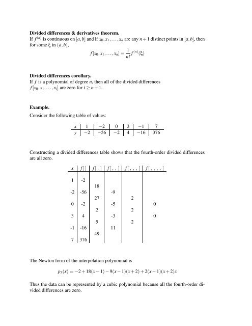
Example.<br />
Consider the following table of values:<br />
x 1 −2 0 3 −1 7<br />
y −2 −56 −2 4 −16 376<br />
Constructing a divided differences table shows that the fourth-order divided differences<br />
are all zero.<br />
x f[] f[, ] f[, , ] f[, , , ] f[, , , , ]<br />
1 -2<br />
18<br />
-2 -56 -9<br />
27 2<br />
0 -2 -5 0<br />
2 2<br />
3 4 -3 0<br />
5 2<br />
-1 -16 11<br />
49<br />
7 376<br />
The Newton form of the <strong>interpolation</strong> polynomial is<br />
p 3 (x)=−2+18(x−1)−9(x−1)(x+2)+2(x−1)(x+2)x<br />
Thus the data can be represented by a cubic polynomial because all the fourth-order divided<br />
differences are zero.