LECTURE 3: Polynomial interpolation and numerical differentiation

LECTURE 3: Polynomial interpolation and
numerical differentiation
October 1, 2012
1 Introduction
An interpolation task usually involves a given set of data points: where the values y i can,
x i x 0 x 1 ... x n
f(x i ) y 0 y 1 ... y n
for example, be the result of some physical measurement or they can come from a long
numerical calculation. Thus we know the value of the underlying function f(x) at the set
of points{x i }, and we want to find an analytic expression for f .
In interpolation, the task is to estimate f(x) for arbitrary x that lies between the smallest
and the largest x i . If x is outside the range of the x i ’s, then the task is called extrapolation,
which is considerably more hazardous.
By far the most common functional forms used in interpolation are the polynomials.
Other choices include, for example, trigonometric functions and spline functions (discussed
later during this course).
Examples of different types of interpolation tasks include:
1. Having the set of n+1 data points {x i ,y i }, we want to know the value of y in the
whole interval x=[x 0 ,x n ]; i.e. we want to find a simple formula which reproduces
the given points exactly.
2. If the set of data points involve errors (e.g. if they are measured values), then we
ask for a formula that represents the data, and if possible, filters out the errors.
3. A function f may be given in the form of a computer procedure which is expensive
to evaluate. In this case, we want to find a function g which gives a good
approximation of f and is simpler to evaluate.

2 Polynomial interpolation
2.1 Interpolating polynomial
Given a set of n+1 data points {x i ,y i }, we want to find a polynomial curve that passes
through all the points. Thus, we look for a continuous curve which takes on the values y i
for each of the n+1 distinct x i ’s.
A polynomial p for which p(x i )=y i when 0≤i≤n is said to interpolate the given set of
data points. The points x i are called nodes.
The trivial case is n=0. Here a constant function p(x)=y 0 solves the problem.
The simplest case is n=1. In this case, the polynomial p is a straight line defined by
( ) ( )
x−x1 x−x0
p(x)= y 0 + y 1
x 0 − x 1 x 1 − x
( ) 0
y1 − y 0
= y 0 + (x−x 0 )
x 1 − x 0
Here p is used for linear interpolation.
As we will see, the interpolating polynomial can be written in a variety of forms, among
these are the Newton form and the Lagrange form. These forms are equivalent in the
sense that the polynomial in question is the one and the same (in fact, the solution to the
interpolation task is given by a unique polynomial)
We begin by discussing the conceptually simpler Lagrange form. However, a straightforward
implementation of this form is somewhat awkward to program and unsuitable for
numerical evaluation (e.g. the resulting algorithm gives no error estimate). The Newton
form is much more convenient and efficient, and therefore, it is used as the basis for
numerical algorithms.
2.2 Lagrange form
First define a system of n+1 special polynomials l i known as cardinal functions. These
have the following property:
{
0 if i≠ j
l i (x j )=δ i j =
1 if i= j
The cardinal functions l i can be written as the product of n linear functions (the variable
x occurs only in the numerator of each term; the denominators are just numbers):
( ) x−x j
l i (x)= (0≤i≤n)
x i − x j
=
n
∏
j≠i
j=0
( )( )
x−x0 x−x1
...
x i − x 0 x i − x 1
Thus l i is a polynomial of degree n.
( )( ) ( )
x−xi−1 x−xi+1 x−xn
...
x i − x i−1 x i − x i+1 x i − x n

Note that when l i (x) is evaluated at x=x i , each factor in the preceding equation becomes
1. But when l i (x) is evaluated at some other node x j , one of the factors becomes 0, and
thus l i (x j )=0 for i≠ j.
Once the cardinal functions are defined, we can interpolate any function f by the following
Lagrange form of the interpolation polynomial:
p n (x)=
n
∑
i=0
l i (x) f(x i )
Writing out the summation, we get
( ) ( ) ( )
x−x1 x−xi x−xn
p n (x)= ... ... f(x 0 ) +...+
x 0 − x 1 x 0 − x i x 0 − x
( )( ) ( )( n
) ( )
x−x0 x−x1 x−xi−1 x−xi+1 x−xn
+ ...
... f(x i ) +...+
x i − x 0 x i − x 1 x i − x i−1 x i − x i+1 x i − x
( ) ( ) ( )
n
x−x0 x−xi x−xn−1
+ ... ...
f(x n )
x n − x 0 x n − x i x n − x n−1
It is easy to check that this function passes through all the nodes, i.e. p n (x j )= f(x j )=y j .
Since the function p n is a linear combination of the polynomials l i , it is itself a polynomial
of degree n or less.
Example.
Find the Lagrange form of the interpolating polynomial for the following table of values:
x 1/3 1/4 1
y 2 −1 7
The cardinal functions are:
l 0 (x)= (x−1/4)(x−1)
(1/3−1/4)(1/3−1) =−18(x−1/4)(x−1)
l 1 (x)= (x−1/3)(x−1)
(1/4−1/3)(1/4−1) = 16(x−1/3)(x−1)
l 2 (x)= (x−1/3)(x−1/4)
(1−1/3)(1−1/4) = 2(x−1/3)(x−1/4)
Therefore, the interpolating polynomial in Lagrange’s form is
p 2 (x)=−36(x−1/4)(x−1)
− 16(x−1/3)(x−1)
+ 14(x−1/3)(x−1/4)

2.3 Existence of interpolating polynomial
Theorem. If points x 0 ,x 1 ,...,x n are distinct, then for arbitrary real values y 0 ,y 1 ,...,y n ,
there is a unique polynomial p of degree≤n such that p(x i )=y i for 0≤i≤n.
The theorem can be proven by inductive reasoning. Suppose that we have succeeded in
finding a polynomial p that reproduces a part of the given set of data points; e.g. p(x i )=y i
for 0≤i≤k.
We then attempt to add another term to p such that the resulting curve will pass through
yet another data point x k+1 . We consider
where c is a constant to be determined.
q(x)= p(x)+c(x−x 0 )(x−x 1 )...(x−x k )
This is a polynomial and it reproduces the first k data points because p does so and the
added term is 0 at each of the points x 0 ,x 1 ,...,x k .
We now adjust the value of c in such a way that the new polynomial q takes the value y k+1
at x k+1 . We obtain
q(x k+1 )= p(x k+1 )+c(x k+1 − x 0 )(x k+1 − x 1 )...(x k+1 − x k )=y k+1
The proper value of c can be obtained from this equation since all the x i ’s are distinct.

2.4 Newton form
The inductive proof of the existence of interpolating polynomial theorem provides a
method for constructing an interpolating polynomial. The method is known as the Newton
algorithm.
The method is based on constructing successive polynomials p 0 , p 1 , p 2 ,... until the desired
degree n is reached (determined by the number of data points = n+1).
The first polynomial is given by
Adding the second term gives
p 0 (x)=y 0
p 1 (x)= p 0 (x)+c 1 (x−x 0 )=y 0 + c 1 (x−x 0 )
Interpolation condition is p 1 (x 1 )=y 1 . Thus we obtain
y 0 + c 1 (x 1 − x 0 )=y 1
which leads to
c 1 = y 1− y 0
x 1 − x 0
The value of c is evaluated and placed in the formula for p 1 .
We then continue to the third term which is given by
p 2 (x)= p 1 (x)+c 2 (x−x 0 )(x−x 1 )=y 0 + c 1 (x−x 0 )+c 2 (x−x 0 )(x−x 1 )
We again impose the interpolation condition p 2 (x 2 )=y 2 and use it to calculate the value
of c.
The iteration for the kth polynomial is
p k (x)= p k−1 (x)+c k (x−x 0 )(x−x 1 )...(x−x k−1 )
In the end we obtain the Newton form of the interpolating polynomial:
p n (x)=a 0 + a 1 (x−x 0 )+a 2 (x−x 0 )(x−x 1 )...+a n (x−x 0 )...(x−x n−1 )
where the coefficients y 0 ,c 1 ,c 2 ,... have been denoted by a i .

Example.
Find the Newton form of the interpolating polynomial for the following table of values:
x 1/3 1/4 1
y 2 −1 7
We will construct three successive polynomials p 0 , p 1 and p 2 . The first one is
p 0 (x)=2
The next one is given by
p 1 (x)= p 0 (x)+c 1 (x−x 0 )=2+c 1 (x−1/3)
Using the interpolation condition p 1 (1/4)=−1, we obtain c 1 = 36, and
p 1 (x)=2+36(x−1/3)
Finally,
p 2 (x)= p 1 (x)+c 2 (x−x 0 )(x−x 1 )
= 2+36(x−1/3)+c 2 (x−1/3)(x−1/4)
The interpolation condition gives p 2 (1)=7, and thus c 2 =−38.
The Newton form of the interpolating polynomial is
p 2 (x)=2+36(x−1/3)−38(x−1/3)(x−1/4)
Comparison of Lagrange and Newton forms
Lagrange form
p 2 (x)=−36(x−1/4)(x−1)
− 16(x−1/3)(x−1)
+ 14(x−1/3)(x−1/4)
Newton form
p 2 (x)=2+36(x−1/3)−38(x−1/3)(x−1/4)
These two polynomials are equivalent, i.e:
p 2 (x)=−38x 2 +(349/6)x−79/6

2.5 Nested multiplication
For efficient evaluation, the Newton form can be rewritten in a so-called nested form. This
form is obtained by systematic factorisation of the original polynomial.
Consider a general polynomial in the Newton form
p n (x)=a 0 + a 1 (x−x 0 )+a 2 (x−x 0 )(x−x 1 )...+a n (x−x 0 )...(x−x n−1 )
This can be written as
p n (x)=a 0 +
n
∑
i=1
[ ]
i−1
a i (x−x j )
∏
j=0
Let us now rewrite the Newton form of the interpolating polynomial in the nested form
by using the common terms(x−x i ) for factoring. We obtain
p n (x)=a 0 +(x−x 0 )(a 1 +(x−x 1 )(a 2 +(x−x 2 )(a 3 +...+(x−x n−1 )a n )...))
This is called the nested form and its evaluation is done by nested multiplication.
When evaluating p(x) for a given numerical value of x = t, we naturally begin with the
innermost parenthesis:
The quantity v n is p(t).
v 0 = a n
v 1 = v 0 (t− x n−1 )+a n−1
v 2 = v 1 (t− x n−2 )+a n−2
.
v n = v n−1 (t− x 0 )+a 0
In the actual implementation, we only need one variable v. The following pseudocode
shows how the evaluation of p(x = t) is done efficiently once the coefficients a i of the
Newton form are known. The array (x i ) 0:n contains the n+1 nodes x i .
real array (a i ) 0:n ,(x i ) 0:n
integer i,n
real t,v
v←a n
for i=n-1 to 0 step -1 do
v←v(t− x i )+a i
end for

2.6 Divided differences
The next step is to discuss a method for determining the coefficients a i efficiently. We start
with a table of values of a function f : We have seen that there exists a unique polynomial
x x 0 x 1 ... x n
f(x) f(x 0 ) f(x 1 ) ... f(x n )
p of degree≤n. In the compact notation of the Newton form p is written as
[ ]
n i−1
p n (x)= a i (x−x j )
∑
i=0
in which ∏ −1
j=0 (x−x j) is interpreted as 1.
Notice that the coefficients a i do not depend on n. In other words, p n is obtained from
p n−1 by adding one more term, without altering the coefficients already present in p n−1 .
A way of systematically determining the coefficients a i is to set x equal to each of the
points x i (0≤i≤n) at a time. The resulting equations are:
⎧
f(x 0 ) = a 0
⎪⎨ f(x 1 ) = a 0 + a 1 (x 1 − x 0 )
In compact form
∏
j=0
f(x 2 ) = a 0 + a 1 (x 2 − x 0 )+a 2 (x 2 − x 0 )(x 2 − x 1 )
⎪⎩
.
f(x k )=
k i−1
∑ a i ∏
i=0 j=0
(x k − x j ) (0≤k≤n)
The coefficients a k are uniquely determined by these equations. The coefficients can now
be solved starting with a 0 which depends on f(x 0 ), followed by a 1 which depends on
f(x 0 ) and f(x 1 ), and so on.
In general, a k depends on the values of f at the nodes x 0 ,...,x k . This dependence is
formally written in the following notation
a k = f[x 0 ,x 1 ,...,x k ]
The quantity f[x 0 ,x 1 ,...,x k ] is called the divided difference of order k for f .
(Suomeksi: jaettu erotus.)

Example. Determine the quantities f[x 0 ], f[x 0 ,x 1 ], and f[x 0 ,x 1 ,x 2 ] for the following table
x 1 -4 0
f(x) 3 13 -23
The system of equations for the coefficients a k :
⎧
⎪⎨ 3 = a 0
13 = a 0 + a 1 (−4−1)
⎪⎩
−23 = a 0 + a 1 (0−1)+a 2 (0−1)(0+4)
We get ⎧
⎪⎨
⎪ ⎩
a 0 = 3
a 1
=[13−a 0 ]/(−4−1)=−2
a 2 =[−23−a 0 − a 1 (0−1)]/(0+4)= 7
Thus for this function, f[1]=3, f[1,−4]=−2, and f[1,−4,0]=7.
With the new notation for divided differences, the Newton form of the interpolating
polynomial takes the form
{
}
i−1
p n (x)= f[x 0 ,x 1 ,...,x i ] (x−x j )
n
∑
i=0
∏
j=0
The required divided differences f[x 0 ,x 1 ,...,x k ] (the coefficients) can be computed recursively.
We can write
f(x k )=
k i−1
∑ a i ∏
i=0 j=0
(x k − x j )
k−1
= f[x 0 ,x 1 ,...,x k ]
∏
j=0
(x k − x j )+
k−1
∑
i=0
i−1
f[x 0 ,x 1 ,...,x i ]
∏
j=0
(x k − x j )
and
f[x 0 ,x 1 ,...,x k ]= f(x k)−∑ k−1
i=0 f[x 0,x 1 ,...,x i ]∏ i−1
j=0 (x k− x j )
∏ k−1
j=0 (x k− x j )
Thus one possible algorithm for computing the divided differences is
i. Set f[x 0 ]= f(x 0 ).
ii. For k=1,2,...,n, compute f[x 0 ,x 1 ,...,x k ] by the equation above.

This can be easily programmed; the algorithm is capable of computing the divided differences
at the cost of 1 2n(3n+1) additions/subtractions,(n−1)(n−2) multiplications, and
n divisions.
There is, however, a more refined method for calculating the divided differences.

2.7 Recursive property of divided differences
The efficient method for calculating the divided differences is based on two properties of
the divided differences.
First, the divided differences obey the formula (the recursive property of divided differences)
f[x 0 ,x 1 ,...,x k ]= f[x 1,x 2 ,...,x k ]− f[x 0 ,x 1 ,...,x k−1 ]
x k − x 0
The proof is left to the student (see e.g., Cheney and Kincaid, pp. 134, Theorem 2).
Second, because of the uniqueness of the interpolating polynomials, the divided differences
are not changed if the nodes are permuted. This is expressed more formally by the
following theorem.
Invariance theorem.
The divided difference f[x 0 ,x 1 ,...,x k ] is invariant under all permutations of the arguments
x 0 ,x 1 ,...,x k .
Thus, the recursive formula can also be written as
f[x i ,x i+1 ,...,x j−1 ,x j ]= f[x i+1,x i+2 ,...,x j ]− f[x i ,x i+1 ,...,x j−1 ]
x j − x i
We can now determine the divided differences as follows:
f[x i ]= f(x i ) f[x i+1 ]= f(x i+1 ) f[x i+2 ]= f(x i+2 )
f[x i ,x i+1 ]= f[x i+1]− f[x i ]
x i+1 − x i
f[x i+1 ,x i+2 ]= f[x i+2]− f[x i+1 ]
x i+2 − x i+1
f[x i ,x i+1 ,x i+2 ] = f[x i+1,x i+2 ]− f[x i ,x i+1 ]
x i+2 − x i

Using the recursive formula, we can now construct a divided-differences table for a function
f
x f[] f[, ] f[, , ] f[, , , ]
x 0 f[x 0 ]
f[x 0 ,x 1 ]
x 1 f[x 1 ] f[x 0 ,x 1 ,x 2 ]
f[x 1 ,x 2 ] f[x 0 ,x 1 ,x 2 ,x 3 ]
x 2 f[x 2 ] f[x 1 ,x 2 ,x 3 ]
f[x 2 ,x 3 ]
x 3 f[x 3 ]
Example.
Construct a divided differences table and write out the Newton form of the interpolating
polynomial for the following table of values:
x i 1 3/2 0 3
f(x i ) 3 13/4 3 5/3
Step 1.
The second column of entries is given by f[x i ]= f(x i ). Thus
x f[] f[, ] f[, , ] f[, , , ]
1 3
f[x 0 ,x 1 ]
3/2 13/4 f[x 0 ,x 1 ,x 2 ]
f[x 1 ,x 2 ] f[x 0 ,x 1 ,x 2 ,x 3 ]
0 3 f[x 1 ,x 2 ,x 3 ]
f[x 2 ,x 3 ]
2 5/3
Step 2.
The third column of entries is obtained using the values in the second column:
f[x i ,x i+1 ]= f[x i+1]− f[x i ]
x i+1 − x i
For example,
f[x 0 ,x 1 ]= f[x 1]− f[x 0 ]
x 1 − x 0
= 13/4−3
3/2−1 = 1 2

The table with a completed second column is
x f[] f[, ] f[, , ] f[, , , ]
1 3
1/2
3/2 13/4 f[x 0 ,x 1 ,x 2 ]
1/6 f[x 0 ,x 1 ,x 2 ,x 3 ]
0 3 f[x 1 ,x 2 ,x 3 ]
-2/3
2 5/3
Step 3.
The first entry in the fourth column is obtained using the values in the third column:
f[x 0 ,x 1 ,x 2 ] = f[x 1,x 2 ]− f[x 0 ,x 1 ]
x 2 − x 0
The table with a completed third column is
x f[] f[, ] f[, , ] f[, , , ]
= 1/6−1/2
0−1
1 3
1/2
3/2 13/4 1/3
1/6 f[x 0 ,x 1 ,x 2 ,x 3 ]
0 3 -5/3
-2/3
2 5/3
= 1 3
Step 4.
The final entry in the table is
The completed table is
f[x 0 ,x 1 ,x 2 ,x 3 ] = f[x 1,x 2 ,x 3 ]− f[x 0 ,x 1 ,x 2 ]
x 3 − x 0
x f[] f[, ] f[, , ] f[, , , ]
1 3
1/2
3/2 13/4 1/3
1/6 -2
0 3 -5/3
-2/3
2 5/3
= −5/3−1/3
2−1
=−2

Using the values shown in bold text in the divided differences table, we can now write out
the Newton form of the interpolating polynomial. We get
{
}
i−1
p n (x)= f[x 0 ,x 1 ,...,x i ] (x−x j )
n
∑
i=0
∏
j=0
= f[x 0 ]+ f[x 0 ,x 1 ](x−x 0 )+ f[x 0 ,x 1 ,x 2 ](x−x 0 )(x−x 1 )
+ f[x 0 ,x 1 ,x 2 ,x 3 ](x−x 0 )(x−x 1 )(x−x 2 )
= 3+ 1 2 (x−1)+ 1 3 (x−1)(x− 3 2 )−2(x−1)(x− 3 2 )x
2.8 Algorithms
We now use the same procedure to construct an algorithm which computes all the divided
differences a i j ≡ f[x i ,x i+1 ,...,x j ].
Notice that there is no need to store all the values in the table since only f[x 0 ], f[x 0 ,x 1 ],..., f[x 0 ,x 1 ,...,x n ]
are needed to construct the Newton form of the interpolating polynomial.
Denote a i ≡ f[x 0 ,x 1 ,...,x i ]. Using this notation, the Newton form is given by
p n (x)=
n i−1
∑ a i ∏
i=0 j=0
(x−x j )
We can use a one-dimensional array (a i ) 0:n for storing the divided differences and overwrite
the entries each time from the last storage location backward. At each step, the new
value of each new divided difference is obtained using the recursion formula:
a i ←(a i − a i−1 )/(x i − x i− j )
where j is the index of the step in question (j=1,. . . ,n).

The following procedure Coefficients calculates the coefficients a i required in the Newton
interpolating polynomial. The input is the number n (degree of the polynomial) and the
arrays for x i , y i and a i (all contain n+1 elements). The arrays x i and y i contain the data
points. a i is the array where the coefficients are to be computed.
void Coefficients(int n, double *x, double *y, double *a)
{
int i, j;
for(i=0; i

The procedure Evaluate returns the value of the interpolating polynomial at point t. The
input is the array x i and the array a i which is obtained using the procedure Coefficients.
Also the value of the point t is given.
double Evaluate(int n, double *x, double *a, double t)
{
int i;
double pt;
pt = a[n];
for(i=n-1; i>=0; i--)
pt = pt*(t-x[i])+a[i];
}
return(pt);
Notice that only the value of t should change in subsequent calls of Evaluate.
These procedures Coefficients and Evaluate can be used to construct a program that determines
the Newton form of the interpolating polynomial for a given function f(x). In
such a program, the procedure Coefficients is called once to determine the coefficients and
then the procedure Evaluate is called as many time as needed to determine the value of
the interpolating polynomial at some given set points of interest.
Example.
In the following example, the task is to find the interpolating polynomial for the function
f(x)=sin(x) at ten equidistant points in the interval [0,1.6875] (these ten points are the
nodes). The value of the resulting polynomial p(x) is then evaluated at 37 equally spaced
points in the same interval and also the absolute error| f(x)− p(x)| is calculated.
Output
The following coefficients for the Newton form of the interpolating polynomial are obtained:
i ai
0 0.00000000
1 0.99415092
2 -0.09292892
3 -0.15941590
4 0.01517217
5 0.00738018
6 -0.00073421
7 -0.00015560
8 0.00001671
9 0.00000181

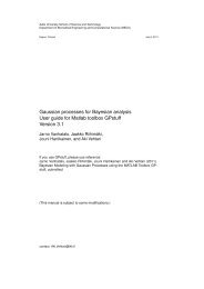
Figure 1 shows a plot of the data points f(x i )=sin(x i ), 0 ≤ i ≤ 9 and the interpolating
polynomial (evaluated at 37 points).
1
0.8
f(x)
0.6
0.4
0.2
0
0 0.5 1 1.5
x
Figure 1: A plot of the original data points (nodes) and the interpolating polynomial.
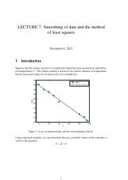
From Fig. 2, we see that the deviation between p(x) and f(x) is zero at each interpolation
node (within the accuracy of the computer). Between the nodes, we obtain deviations that
are less than 5×10 −10 in magnitude.

6 x 10-10
5
4
3
2
1
0
0 5 10 15 20 25 30 35
Figure 2: The absolute error| f(x)− p(x)| between the interpolating polynomial p and the
underlying function f at the 37 interpolation points.

2.9 Inverse interpolation
A process called inverse interpolation can be used to approximate an inverse function.
Suppose that the values y i = f(x i ) have been computed at x 0 ,x 1 ,...,x n .
We can form the interpolation polynomial as
p(y)=
n i−1
∑ c i ∏
i=0 j=0
(y−y j )
The original relationship y = f(x) has an inverse under certain conditions. This can be
approximated by x= p(y).
The procedures Coefficients and Evaluate can be used to carry out the inverse interpolation
by reversing the arguments x and y.
Inverse interpolation can be used to locate the root of a given function f ; i.e. we want to
solve f(x)=0. First create a set of function values { f(x i ),x i } and find the interpolating
polynomial p(y i )=x i .
The approximate root is now given by r≈ p(y=0).
Example.
Having the following set of values
y x
-0.57892000 1.00000000
-0.36263700 2.00000000
-0.18491600 3.00000000
-0.03406420 4.00000000
0.09698580 5.00000000
We can use the interpolation program with
x←y and y←x.
This gives us the coefficients for the polynomial p(y).
Evaluating p at point y=0, gives p(0)=4.24747001.

2.10 Neville’s algorithm
Another widely used method for obtaining the interpolating polynomial for a given table
of values is given by Neville’s algorithm. It builds up the polynomial in steps, just as the
Newton algorithm does.
Let P a,b,...,s be the polynomial interpolating the given data at a sequence of nodes x a ,x b ,...,x s .
We start with constant polynomials P i (x)= f(x i ). Selecting two nodes x i and x j with i> j,
we define recursively
( ) ( )
x−x j
xi − x
P u,...,v (x)= P u,..., j−1, j+1,...,v (x)+ P u,...,i−1,i+1,...,v (x)
x i − x j x i − x j
For example, the first three constant polynomials are
P 0 (x)= f(x 0 ) P 1 (x)= f(x 1 ) P 2 (x)= f(x 2 )
Using P 0 and P 1 , we can construct P 0,1 :
( ) ( )
x−x0 x1 − x
P 0,1 (x)= P 1 + P 0
x 1 − x 0 x 1 − x 0
and similarly
P 1,2 (x)=
( ) ( )
x−x1 x2 − x
P 2 + P 1
x 2 − x 1 x 2 − x 1
Using these two polynomials of degree one, we can construct another polynomial of degree
two: ( ) ( )
x−x0 x2 − x
P 0,1,2 (x)= P 1,2 + P 0,1
x 2 − x 0 x 2 − x 0
Similarly,
P 0,1,2,3 (x)=
( ) ( )
x−x0
x3 − x
P 1,2,3 + P 0,1,2
x 3 − x 0 x 3 − x 0
Using this formula repeatedly, we can create an array of polynomials:
x 0
x 1
x 2
x 3
x 4
P 0 (x)
P 1 (x) P 0,1 (x)
P 2 (x) P 1,2 (x) P 0,1,2 (x)
P 3 (x) P 2,3 (x) P 1,2,3 (x) P 0,1,2,3 (x)
P 4 (x) P 3,4 (x) P 2,3,4 (x) P 1,2,3,4 (x) P 0,1,2,3,4 (x)
Here each successive polynomial can be determined from two adjacent polynomials in
the previous column.

We can simplify the notation by
S i j (x)=P i− j,i− j+1,...,i−1,i (x)
where S i j (x) for i≥ j denotes the interpolating polynomial of degree j on the j+ 1 nodes
x i− j ,x i− j+1 ,...,x i−1 ,x i . For example, S 44 is the interpolating polynomial of degree 4 on
the five nodes x 0 ,x 1 ,x 2 ,x 3 and x 4 .
Using this notation, we can rewrite the recurrence relation as
( ) ( )
x−xi− j
xi − x
S i j (x)=
S i, j−1 (x)+
S i−1, j−1 (x)
x i − x i− j x i − x i− j
The array becomes
x 0
x 1
x 2
x 3
x 4
S 00 (x)
S 10 (x) S 11 (x)
S 20 (x) S 21 (x) S 22 (x)
S 30 (x) S 31 (x) S 32 (x) S 33 (x)
S 40 (x) S 41 (x) S 42 (x) S 43 (x) S 44 (x)
Algorithm
A pseudocode to evaluate S nn (x) at point x=t can be written as follows:
real array (x i ) 0:n ,(y i ) 0:n ,(S i j ) 0:n×0:n
integer i, j,n
for i=0 to n
S i0 ← y i
end for
for j=1 to n
for i=j to n
S i j ←[(t− x i− j )S i, j−1 +(x i −t)S i−1, j−1 ]/(x i − x i− j )
end for
end for
return S nn
Here (x i ) 0:n and (y i ) 0:n are the arrays containing the initial data points, and the procedure
returns the value of the interpolating polynomial at point x=t.

3 Errors in polynomial interpolation
When a function f is approximated on an interval [a,b] by an interpolating polynomial
p, the discrepancy between f and p will be zero at each node, i.e., p(x i ) = f(x i ) (at
least theoretically). Based on this, it is easy to expect that when the number of nodes n
increases, the function f will be better approximated at all intermediate points as well.
This is wrong. In many cases, high-degree polynomials can be very unsatisfactory representations
of functions even if the function is continuous and well-behaved.
Example. Consider the Runge function:
f(x)= 1
1+x 2
on the interval [-5,5]. Let p n be the polynomial that interpolates this function at n+1
equally spaced points on the interval [-5,5]. Then
lim
max
n→∞−5≤x≤5 | f(x)− p(x)|=∞
Thus increasing the number of node points increases the error at nonnodal points beyond
all bounds! Figure 3 below shows f and p for n=9.
1
0.8
0.6
0.4
0.2
0
-0.2
-0.4
-5 0 5
Figure 3: The Runge function f (shown in dashed line) and the polynomial interpolant p
obtained using 9 equidistant nodes.

3.1 Choice of nodes
Contrary to intuition, equally distributed nodes are usually not the best choice in interpolation.
A much better choice for n+1 nodes in [-1,1] is the set of Chebyshev nodes:
[( ] i
x i = cos π (0≤i≤n)
n)
The corresponding set of nodes on an arbitrary interval [a,b] can be derived from a linear
mapping to obtain
x i = 1 2 (a+b)+ 1 [ ] i
2 (b−a)cos n π (0≤i≤n)
Notice that the Chebyshev nodes are numbered from right to left (i.e.the largest value has
the lowest index).
Figure 4 shows the polynomial interpolant of the Runge function obtained with 13 Chebyshev
nodes.
1
0.8
0.6
0.4
0.2
0
-0.2
-0.4
-5 0 5
Figure 4: The Runge function f (shown in dashed line) and the polynomial interpolant p
obtained using 13 Chebyshev nodes.

3.2 Theorems on interpolation errors
Theorem 1.
If p is the polynomial of degree at most n that interpolates f at the n+1 distinct nodes
x i (0 ≤ i ≤ n) belonging to an interval [a,b] and if f (n+1) (the nth derivative of f ) is
continuous, then for each x in [a,b], there is a ξ in(a,b) for which
1
f(x)− p(x)=
(n+1)! f(n+1) (ξ)
n
∏
i=0
(x−x i )
Theorem 2.
Let f be a function such that f (n+1) is continuous on [a,b] and satisfies | f (n+1) (x)|≤M.
Let p be the polynomial of degree ≤ n that interpolates f at n+1 equally spaced nodes
in[a,b], including the endpoints. Then on[a,b],
| f(x)− p(x)|=
( )
1 b−a n+1
4(n+1) M n
Theorem 3.
If p is the polynomial of degree n that interpolates the function f at nodes x i (0≤i≤n),
then for any x not a node
f(x)− p(x)= f[x 0 ,x 1 ,...,x n ,x]
n
∏
i=0
(x−x i )

Example.
In a previous example, we constructed the interpolating polynomial of f(x) = sin(x) at
ten equidistant points in [0,1.6875].
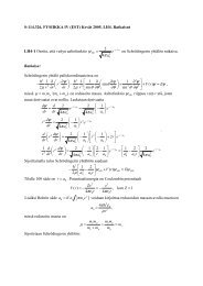
Figure 5 shows a plot of the computed error | f(x)− p(x)|. At the largest, the error is
approximately 5×10 −10 .
6 x 10-10
5
4
3
2
1
0
0 5 10 15 20 25 30 35
Figure 5: The absolute error | f(x)− p(x)| in polynomial interpolation of f(x) = sin(x)
using ten equidistant nodes.
Now use Theorem 2 with f(x)=sin(x), n=9, a=0and b=1.6875. The 10th derivative
of f is f (10) (x)=−sin(x), and thus| f (10) (x)|≤1. Thus we can let M = 1.
The resulting bound for the error is
| f(x)− p(x)|≤
( )
1 b−a n+1
4(n+1) M = 1.34×10 −9
n

Divided differences & derivatives theorem.
If f (n) is continuous on[a,b] and if x 0 ,x 1 ,...,x n are any n+1 distinct points in[a,b], then
for some ξ in (a,b),
f[x 0 ,x 1 ,...,x n ]= 1 n! f(n) (ξ)
Divided differences corollary.
If f is a polynomial of degree n, then all of the divided differences
f[x 0 ,x 1 ,...,x i ] are zero for i≥n+1.
Example.
Consider the following table of values:
x 1 −2 0 3 −1 7
y −2 −56 −2 4 −16 376
Constructing a divided differences table shows that the fourth-order divided differences
are all zero.
x f[] f[, ] f[, , ] f[, , , ] f[, , , , ]
1 -2
18
-2 -56 -9
27 2
0 -2 -5 0
2 2
3 4 -3 0
5 2
-1 -16 11
49
7 376
The Newton form of the interpolation polynomial is
p 3 (x)=−2+18(x−1)−9(x−1)(x+2)+2(x−1)(x+2)x
Thus the data can be represented by a cubic polynomial because all the fourth-order divided
differences are zero.

4 Numerical differentiation
We now move on to a slightly different subject, namely numerical differentiation. This
subject is often not discussed in great detail, but we include it here because the central
idea of a process called Richardson extrapolation is also used in numerical integration.
Determining the derivative of a function f at point x is not a trivial numerical problem.
Specifically, if f(x) can be computed with n digits of precision, it is difficult to calculate
f ′ (x) numerically with n digits of precision. This is caused by subtraction of nearly equal
quantities (loss of precision).
4.1 First-derivative formulas via Taylor series
Consider first the obvious method based on the definition of f ′ (x):
f ′ (x)≈ 1 [ f(x+h)− f(x)]
h
What is the error involved in this formula? By Taylor’s theorem:
Rearranging this gives:
f(x+h)= f(x)+h f ′ (x)+ 1 2 h2 f ′′ (ξ)
f ′ (x)= 1 h [ f(x+h)− f(x)]− 1 2 h f′′ (ξ)
We see that the first approximation has a truncation error − 1 2 h f′′ (ξ) where ξ is in the
interval [x,x+h]. In general, as h → 0, the error approaches zero at the same rate as h
does - that is O(h).
It is advantageous to have the convergence of numerical processes occur with high powers
of some quantity approaching zero. In the present case, we want an approximation to f ′ (x)
in which the error behaves like O(h 2 ).
One such method is obtained using the following two Taylor series:
{
f(x+h)= f(x)+h f ′ (x)+ 1 2! h2 f ′′ (x)+ 1 3! h3 f ′′′ (x)+ 1 4! h3 f (4) (x)+...
f(x−h)= f(x)−h f ′ (x)+ 1 2! h2 f ′′ (x)− 1 3! h3 f ′′′ (x)+ 1 4! h4 f (4) (x)−...
By subtraction, we obtain
f(x+h)− f(x−h)=2h f ′ (x)+ 2 3! h3 f ′′′ (x)+ 2 5! h5 f (5) (x)+...
From this we obtain the following formula for f ′ :
f ′ (x)= 1
2h [ f(x+h)− f(x−h)]− 1 3! h2 f ′′′ (x)− 1 5! h4 f (5) (x)−...

Thus we obtain an approximation formula for f ′ with an error whose leading term is
− 1 6 h2 f ′′′ (x), which makes it O(h 2 ):
f ′ (x)≈ 1 [ f(x+h)− f(x−h)]
2h
The approximation formula with the error term can be written as
f ′ (x)≈ 1
2h [ f(x+h)− f(x−h)]− 1 6 h2 f ′′′ (ξ)
where ξ is some point on the interval [x−h,x+h]. This is based only on the assumption
that f ′′′ is continuous on[x−h,x+h].
4.2 Richardson extrapolation
Richardson extrapolation is a powerful technique for obtaining accurate results from a
numerical process such as the approximation formula for f ′ obtained via Taylor series:
f ′ (x)≈ 1
2h [ f(x+h)− f(x−h)]+a 2h 2 + a 4 h 4 + a 6 h 6 +...
where the constants a i depend on f and x.
Holding f and x fixed, we define a function of h by the formula
ϕ(h)≈ 1 [ f(x+h)− f(x−h)]
2h
where ϕ(h) is an approximation to f ′ (x) with an error of order O(h 2 ).
Our objective is to compute the limit lim h→0 ϕ(h) because this is the quantity f ′ (x). Since
we cannot actually compute the value of ϕ(0) from the equation above, Richardson extrapolation
seeks to estimate the limiting value at 0 from some computed values of ϕ near
0.
Suppose now that we compute ϕ(h) and ϕ(h/2) for some h:
{
ϕ(h)= f ′ (x)−a 2 h 2 − a 4 h 4 − a 6 h 6 −...
ϕ( h 2 )= f′ (x)−a 2
( h2
) 2−
a4
( h2
) 4−
a6
( h2
) 6−...
We can now use simple algebra to eliminate the dominant term in the error series. We
multiply the bottom series by 4 and subtract it from the top equation. The result is
ϕ(h)−4ϕ( h 2 )=−3 f′ (x)− 3 4 a 4h 4 − 15
16 a 6h 6 −...
Divide this by -3 and rearrange to get
ϕ( h 2 )+ 1 [ϕ( h ]
3 2 )−ϕ(h) = f ′ (x)+ 1 4 a 4h 4 + 5
16 a 6h 6 +...
Thus we have improved the precision to O(h 4 )!! The same procedure can be repeated over
and over again to "kill" higher order terms from the error series. This is called Richardson
extrapolation.

4.3 Richardson extrapolation theorem
The same procedure will be needed later in the derivation of the Romberg’s algorithm for
numerical integration. We therefore want to have a general discussion of the procedure.
Let ϕ be a function such that
ϕ(h)=L−
∞
∑
k=1
a 2k h 2k
where the coefficients a 2k are not known. It is assumed that ϕ(h) can be computed accurately
for any h>0. Our objective is to approximate L accurately using ϕ.
We select a convenient h and compute the numbers
We have
D(n,0)= ϕ( h 2n) (n≥0)
D(n,0)=L+
∞
∑
k=1
( ) h 2k
A(k,0)
2 n
where A(k,0)=−a 2k . These numbers D(n,0) give a crude estimate of the unknown number
L=lim x→0 ϕ(x).
More accurate estimates are obtained via Richardson extrapolation:
D(n,m)= 4m
4 m − 1 D(n,m−1)− 1
4 m − 1 D(n−1,m−1)
This is called the Richardson extrapolation formula.
Theorem.
The quantities D(n,m) obey the equation
D(n,m)=L+
∞
∑
k=m+1
A(k,m)( h
2 n ) 2k
(0≤m≤n)
4.4 Algorithm for Richardson extrapolation
1. Write a procedure function for ϕ.
2. Decide suitable values for N and h.
3. For i=0,1,...,N, compute D(i,0)= ϕ(h/2 i ).
4. For 0≤i≤ j≤ N, compute
D(i, j)=D(i, j− 1)+(4 j − 1) −1 [D(i, j− 1)−D(i−1, j− 1)].
In this algorithm the computation of D(i, j) has been rearranged slightly to improve its
numerical properties.

Example
The Richardson extrapolation algorithm is implemented in the following procedure Derivative:
void Derivative(double (*f)(double x), double x,
int n, double h, double D[][NCOLS])
{
int i, j;
double hh;
}
hh=h;
for(i=0; i

4.5 First-derivative formulas via interpolation polynomials
An important stratagem can be used to approximate derivatives (as well as integrals and
other quantities). The function f is first approximated by a polynomial p. Then we simply
approximate the derivative of f by the derivative of p: f ′ (x)≈ p ′ (x). Of course, we must
be careful with this strategy because the behavior of p may be oscillatory.
In practice, the approximating polynomial is often determined by interpolation at a few
points. For two nodes, we have
Consequently,
p 1 (x)= f(x 0 )+ f[x 0 ,x 1 ](x−x 0 )
f ′ (x)≈ p ′ (x)= f[x 0 ,x 1 ]= f(x 1)− f(x 0 )
x 1 − x 0
If x 0 = x and x 1 = x+h, this formula gives
If x 0 = x−h and x 1 = x+h, we get
f ′ (x)≈ 1 [ f(x+h)− f(x)]
h
f ′ (x)≈ 1 [ f(x+h)− f(x−h)]
2h
Now consider interpolation at three nodes
The derivative is
p 2 (x)= f(x 0 )+ f[x 0 ,x 1 ](x−x 0 )+ f[x 0 ,x 1 ,x 2 ](x−x 0 )(x−x 1 )
p ′ 2(x)= f[x 0 ,x 1 ]+ f[x 0 ,x 1 ,x 2 ](2x−x 0 − x 1 )
Here the first term is the same as in the previous case and the second term is a refinement
or a correction term.
The accuracy of the leading term depends on the choice of the nodes x 0 and x 1 . If we
have x=(x 0 + x 1 )/2, then the correction term is zero. Thus the first term must be more
accurate than in other cases. This is why choosing a central difference x 0 = x−h and
x 1 = x+h gives more accurate results than x 0 = x and x 1 = x+h.

In general, an analysis of errors goes as follows: Suppose that p n is the polynomial of
least degree that interpolates f at the nodes x 0 ,x 1 ,...,x n . Then according to first theorem
on interpolating errors (Sec.3.2):
f(x)− p n (x)=
1
(n+1)! f(n+1) (ξ)w(x)
with ξ dependent on x and w(x)=(x−x 0 )...(x−x n ). Differentiating gives
f ′ (x)− p ′ n(x)=
1
(n+1)! w(x) d 1
dx f(n+1) (ξ)+
(n+1)! f(n+1) (ξ)w ′ (x)
The first observation is that w(x) vanishes at each node. The evaluation is simpler if it is
done at a node x i :
f ′ (x i )= p ′ 1
n(x i )+
(n+1)! f(n+1) (ξ)w ′ (x i )
The second observation is that it becomes simpler if x is chosen such that w ′ (x)=0. Then
f ′ (x i )= p ′ n (x i)+
1
(n+1)! w(x) d dx f(n+1) (ξ)
Example.
Derive a first-derivative formula for f ′ (x) using an interpolating polynomial p 3 (x) obtained
with four nodes x 0 , x 1 , x 2 and x 3 . Use central difference in choosing the nodes.
Solution. The interpolating polynomial written in the Newton form is
Its derivative is
p 3 (x)= f(x 0 )+ f[x 0 ,x 1 ](x−x 0 )+ f[x 0 ,x 1 ,x 2 ](x−x 0 )(x−x 1 )
+ f[x 0 ,x 1 ,x 2 ,x 3 ](x−x 0 )(x−x 1 )(x−x 2 )
p ′ 3 (x)= f[x 0,x 1 ]+ f[x 0 ,x 1 ,x 2 ](2x−x 0 − x 1 )
+ f[x 0 ,x 1 ,x 2 ,x 3 ]{(x−x 1 )(x−x 2 )+(x−x 0 )(x−x 2 )
+(x−x 0 )(x−x 1 )}
Formulas for the divided differences can be obtained
recursively:
f[x i ]= f(x i )
f[x i ,x i+1 ]= f[x i+1]− f[x i ]
x i+1 − x i
f[x i ,x i+1 ,x i+2 ] = f[x i+1,x i+2 ]− f[x i ,x i+1 ]
x i+2 − x i
We now choose the nodes using central difference:
x 0 = x−h, x 1 = x+h, x 2 = x−2h, x 3 = x+2h.

This allows us to write out the formulas for the divided
differences:
f[x 0 ,x 1 ]= f(x 1)− f(x 0 )
x 1 − x 0
=
f(x+h)− f(x−h)
2h
and
f[x 0 ,x 1 ,x 2 ]= f[x 1,x 2 ]− f[x 0 ,x 1 ]
x 2 − x 1
= 1 [ ]
f(x−2h)− f(x+h) f(x+h)− f(x−h)
−
−h −3h
2h
= 1
6h2[2 f(x−2h)−3 f(x−h)+ f(x+h)]
Similarly for f[x 1 ,x 2 ,x 3 ].
Finally, we obtain
f[x 0 ,x 1 ,x 2 ,x 3 ]=
1
12h3[ f(x+2h)−2 f(x+h)+2 f(x−h)− f(x−2h)]
The two remaining factors in the equation for p 3 are
and
(2x−x 0 − x 1 )=2x−x+h−x−h=0
(x−x 1 )(x−x 2 )+(x−x 0 )(x−x 2 )+(x−x 0 )(x−x 1 )=
− 2h 2 + 2h 2 − h 2 =−h 2
The resulting formula is
f ′ (x)≈ 1 [ f(x+h)− f(x−h)]
2h
− 1 [ f(x+2h)−2 f(x+h)+2 f(x−h)− f(x−2h)]
12h

Numerical evaluation
The obtained formula
f ′ (x)≈ 1 [ f(x+h)− f(x−h)]
2h
− 1 [ f(x+2h)−2 f(x+h)+2 f(x−h)− f(x−2h)]
12h
can be used in the Richardson extrapolation algorithm to speed up the convergence. As
an example, the algorithm is applied to evaluate f ′ at x=1.2309594154 for f(x)=sin(x)
and h=1.
We obtain the following output:
D(n,0) D(n,1) D(n,2) D(n,3) D(n,4)
0.32347058
0.33265926 0.33572215
0.33329025 0.33350059 0.33335248
0.33333063 0.33334409 0.33333365 0.33333335
0.33333317 0.33333401 0.33333334 0.33333334 0.33333334
Using the original formula (first term of the equation above)
D(n,0) D(n,1) D(n,2) D(n,3) D(n,4)
0.28049033
0.31961703 0.33265926
0.32987195 0.33329025 0.33333232
0.33246596 0.33333063 0.33333332 0.33333333
0.33311636 0.33333317 0.33333333 0.33333334 0.33333334
Notice that the first column of the first output has the same values as the second column
of the second output! This is a good example of how the Richardson algorithm works in
refining the approximation.