Modified Fisher's Linear Discriminant Analysis for ... - IEEE Xplore

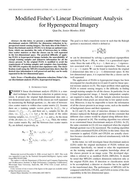
IEEE GEOSCIENCE AND REMOTE SENSING LETTERS, VOL. 4, NO. 4, OCTOBER 2007 503
Modified Fisher’s Linear Discriminant Analysis
for Hyperspectral Imagery
Qian Du, Senior Member, IEEE
Abstract—In this letter, we present a modified Fisher’s linear
discriminant analysis (MFLDA) for dimension reduction in hyperspectral
remote sensing imagery. The basic idea of the Fisher’s
linear discriminant analysis (FLDA) is to design an optimal transform,
which can maximize the ratio of between-class to withinclass
scatter matrices so that the classes can be well separated
in the low-dimensional space. The practical difficulty of applying
FLDA to hyperspectral images includes the unavailability of
enough training samples and unknown information for all the
classes present. So the original FLDA is modified to avoid the
requirements of training samples and complete class knowledge.
The MFLDA requires the desired class signatures only. The classification
result using the MFLDA-transformed data shows that the
desired class information is well preserved and they can be easily
separated in the low-dimensional space.
Index Terms—Classification, dimension reduction, Fisher’s linear
discriminant analysis (FLDA), hyperspectral imagery.
I. INTRODUCTION
FISHER’S linear discriminant analysis (FLDA) is a standard
technique for dimension reduction in pattern recognition.
It projects the original high-dimensional data onto a
low-dimensional space, where all the classes are well separated
by maximizing the Raleigh quotient, i.e., the ratio of betweenclass
scatter matrix to within-class scatter matrix [1]. Assume
there are n training sample vectors given by {r i } n i=1 for p
classes: C 1 ,C
∑ 2 ,...,C p , and there are n j samples for the jth
class, i.e., p
j=1 n j = n. Let µ be the mean of the entire
training samples, i.e., (1/n) ∑ n
i=1 r i = µ, and µ j be the mean
of the jth class, i.e., (1/n j ) ∑ r i ∈C j
r i = µ j . Then, the withinclass
scatter matrix S W and the between-class scatter matrix
S B are defined, respectively, as
S W = ∑
(r i − µ j )(r i − µ j ) T (1)
r i ∈C j
p∑
S B = n j (µ j − µ)(µ j − µ) T . (2)
j=1
Manuscript received December 8, 2006; revised April 21, 2007. This work
was supported in part by the National Geospatial-Intelligence Agency under
Grant HM15810512006.
The author is with the Department of Electrical and Computer Engineering
and GeoResources Institute in High Performance Computing Collaboratory,
Mississippi State University, Starkville, MS 39762 USA (e-mail: du@ece.
msstate.edu).
Color versions of one or more of the figures in this paper are available online
at http://ieeexplore.ieee.org.
Digital Object Identifier 10.1109/LGRS.2007.900751
The goal is to find a transform vector w such that the Raleigh
quotient is maximized, which is defined as
q = wT S B w
w T S W w . (3)
w can be determined by solving a generalized eigenproblem
specified by S B w = λS W w, where λ is a generalized eigenvalue.
Since the rank of S B is p − 1, there are p − 1 eigenvectors
associated with p − 1 nonzero eigenvalues. Therefore, an
L × (p − 1) matrix W can be found to transform the original
L-dimensional data into a (p − 1)-dimensional space. In this
low-dimensional space, it is expected that the p classes can be
well separated.
The application of FLDA to hyperspectral images has been
investigated for classification in [2] and [3] and for linear spectral
mixture analysis in [5]. The major problem when applying
FLDA to remote sensing imagery is the difficulty in finding
enough training samples for all the classes. In particular, for an
L-band hyperspectral image, L linearly independent samples
are required to make S W full rank. Sample selection becomes
very difficult when pixels are mixed due to low spatial resolution.
Moreover, it may be impossible to know the information
of all the classes present in an image scene, such as the number
of background classes and their signatures.
In [2] and [3], the ratio of interclass distance to intraclass
distance replaced the Raleigh quotient with the constraint that
different class centers would be aligned along different directions
as proposed in [4]. The resulting algorithm was referred
to as constrained linear discriminant analysis (CLDA). In [5],
the same constraint in [2]–[4] was employed when the original
Raleigh quotient was to be maximized. The resulting algorithm
was called constrained FLDA (CFLDA) in this letter. Since the
constraint is applied, CLDA and CFLDA are actually classifiers
because classification is achieved simultaneously with the
transforms.
In this letter, we will investigate linear discriminant analysis
(LDA) under the original mechanism of FLDA without any
constraint. Specifically, we intend to relax the requirements
on the training samples and complete knowledge about all
the classes present in an image scene. The developed algorithm
is referred to as modified FLDA (MFLDA). It should
be noted that MFLDA conducts dimension reduction only as
the original FLDA does. If detection or classification needs
to be accomplished, a detector or classifier has to be applied
to the transformed data. The performance of MFLDA will be
compared with FLDA, CFLDA, and CLDA in terms of the class
separability in the low-dimensional space.
1545-598X/$25.00 © 2007 IEEE

504 IEEE GEOSCIENCE AND REMOTE SENSING LETTERS, VOL. 4, NO. 4, OCTOBER 2007
II. MFLDA
Let the total scatter matrix S T be defined as
S T =
n∑
(r i − µ)(r i − µ) T (4)
i=1
and it can be related with S W and S B by [1]
S T = S W + S B . (5)
So the maximization of (3) is equivalent to maximizing
q ′ = wT S B w
w T S T w . (6)
Following the same idea of FLDA, the solution will be the
eigenvectors of the generalized eigenproblem: S B w = λS T w.
When the only available information is the class signatures
{s 1 , s 2 ,...,s p }, they can be treated as class means, i.e., M =
[µ 1 µ 2 ···µ p ] ≈ [s 1 s 2 ···s p ].TheS B in (2) becomes
Ŝ B =
p∑
(s j − ˆµ)(s j − ˆµ) T (7)
j=1
where ˆµ is the mean of class signatures, i.e., (1/p) ∑ p
i=1 s i =
ˆµ. S T in (4) can be replaced by the data covariance
matrix Σ, i.e.,
Ŝ T =Σ=
N∑
(r i − ˜µ)(r i − ˜µ) T (8)
i=1
where ˜µ is the sample mean of the entire data set with N pixels,
i.e., (1/N ) ∑ N
i=1 r i = ˜µ. Then, the solution is the eigenvectors
of the generalized eigenproblem: ŜBw = λΣw or Σ −1 Ŝ B .
Regardless of the actual classes present in the data, replacing
S T with Σ represents an extreme case, which means all the
pixels are separated into the classes they belong to and selected
as samples. Using ŜB as S B represents another extreme case,
which means there is only one sample in each class. So the
discrepancy incurred comes from two factors: only one sample
(i.e., class signature) for each of the p classes is used to estimate
S B , and all the pixels are used to estimate S T with the implicit
assumption that pixels are put into all the existing classes
including unknown background classes (i.e., the actual number
of classes p T may be greater than p). In the experiments, it will
be shown that the term Σ −1 is very effective in background
suppression.
Since the rank of ŜB is the same as S B , which is (p − 1),
the dimensionality of the MFLDA-transformed data is (p − 1)
as that of FLDA. After the data are projected onto this (p − 1)-
dimensional space, an algorithm is needed for some tasks, such
as classification or detection. A less powerful distance-based
classifier such as the Spectral Angle Mapper (SAM) can be
applied. Or, a more powerful filter, such as target constrained
interference minimized filter (TCIMF), may be used [6].
III. RELATIONSHIP BETWEEN LDA-BASED APPROACHES
A. Relationship Between FLDA and CFLDA
The CFLDA in [5] imposed a constraint to align the class
centers along with different directions [4], i.e.,
w T l µ j = δ lj , for 1 ≤ l; j ≤ p. (9)
This also means that the jth transform vector w j is for the
jth class. So the CFLDA-transformed data are actually classification
maps. It can be derived that when the constraint
was satisfied, w T S B w was a constant. Thus, the constrained
problem would be to minimize w T S W w in (3) while satisfying
the constraint in (9). Using the Lagrange multiplier approach,
it was shown that the desired transform matrix W including all
the p transform vectors is
W CFLDA = S −1
W M ( M T S −1
W M) −1
. (10)
Obviously, the implementation of CFLDA requires the
knowledge of the training samples of each class to compute
S W .
B. Relationship Between CFLDA, CLDA, and MFLDA
Following the same idea of FLDA in maximizing the class
separability, the CLDA in [2] and [3] imposed the same
constraint that different classes were aligned along different
directions as in (9). To make the constrained problem easier to
solve, it employed the ratio of within-class and between-class
distances instead of the Raleigh quotient [4]. It was proved that
the transformed within-class distance is a constant when the
constraint in (9) was satisfied. It also used the data covariance
matrix Σ to substitute S T as in MFLDA. It was proved that the
transform matrix W is equivalent to [3]
W CLDA =Σ −1 M(M T Σ −1 M) −1 . (11)
Equation (11) is similar to (10) except that S W is replaced
with Σ. Therefore, CLDA does not require the training samples
in each class and it needs the class signatures only. Similar to
CFLDA, CLDA was designed for classification, so the classification
maps were obtained right after the transform.
C. Use of Σ and S W
Both CFLDA and CLDA apply the constraint in (9), resulting
in the similar operators in (10) and (11) with the difference
that CLDA uses Σ while CFLDA uses S W . So CLDA does
not require the training samples, which is the same as in
MFLDA. There is another benefit of using Σ. As mentioned
earlier, the true number of classes present in an image scene
p T is greater than p due to the difficulty of exhausting all the
present classes, in particular, those background classes. In the
ideal case when all the pixels in an image scene are put into
the p T classes, S T =Σ. Therefore, using Σ in LDA-based
approaches represents the best situation for S T , which means

DU: MODIFIED FISHER’S LINEAR DISCRIMINANT ANALYSIS FOR HYPERSPECTRAL IMAGERY 505
Fig. 1. (a) HYDICE image scene with 30 panels. (b) Spatial locations of the
30 panels that were provided by ground truth.
all the classes can be well separated without knowing these
class information. This is particularly important to suppress
the background classes for better extraction of the foreground
classes. Σ −1 represents the data whitening term, which has
the power to suppress the unknown background classes [7].
Therefore, in general it is reasonable and desirable to use Σ
to replace S W or S T in the practical implementation of LDA.
IV. EXPERIMENTS
A. HYDICE
The HYperspectral Digital Imagery Collection Experiment
(HYDICE) image scene shown in Fig. 1 includes 30 panels
arranged in a 10 × 3 matrix [3]. The three panels in the same
row, i.e., p ia , p ib , p ic , were made from the same material of
sizes 3 m × 3m,2m× 2m,and1m× 1 m, respectively,
which can be considered as one class, P i for 1 ≤ i ≤ 10. The
pixel-level ground truth map in Fig. 1(b) shows the precise
locations of pure panel pixels. These panel classes have very
close signatures for differentiation.
A pure pixel from each leftmost panel (3 m × 3m)was
used as the corresponding class signature. Fig. 2(a) shows the
classification result using SAM on the original data, where
the panels could not be classified. Here, the minimum angle
was displayed in white, the maximum angle in black,
and others in shades between white and black. Fig. 2(b)
is the result using TCIMF, which is a more powerful filter,
on the original image, where the panels were well detected
and separated. Fig. 2(c) shows the SAM classification
result using the 9-D MFLDA-transformed data, where the
panels were correctly classified. This demonstrates that
MFLDA successfully separated the ten panel classes when
performing dimension reduction, allowing a less powerful classifier,
such as SAM, to correctly classify these classes, which is
impossible when using the original 169-D data.
To quantify the performance of MFLDA and compare it with
that of TCIMF using the original data, each classification map
was normalized to [0 1] and converted to a binary map with a
threshold η. The binary classification maps were compared with
the pure panel pixels provided as ground truth. The accurately
detected panel pixels were counted as N D and false alarm as
N F . To comprehensively evaluate the performance, the similar
concept of receiver operating characteristic (ROC) curve was
adopted here [8]. As η was changed from 0.1 to 0.9, an ROC
curve could be estimated. For the 28-pixel test set, the resulting
ROCs with the averaged probability of false alarm (Pf) and
Fig. 2. Comparison between the classification results using the original and
MFLDA-transformed data. (a) SAM (soft) classification result on the original
data. (b) TCIMF (soft) classification result on the original data. (c) SAM (soft)
classification result on the MFLDA-transformed data.
probability of detection (Pd) are shown in Fig. 3. The larger
the area under a curve, the better the performance [9]. We
can see that SAM on the MFLDA-transformed data slightly
outperforms TCIMF on the original data.
To further compare the results in Fig. 2, Table I lists the
largest number of detected pixels in the test set (N D ) when no
false alarm exists (N F =0). This happened when η =0.6 for
the MFLDA with SAM and η =0.4 for TCIMF. By applying
MFLDA followed by SAM, 21 out of 28 panel pixels in the

506 IEEE GEOSCIENCE AND REMOTE SENSING LETTERS, VOL. 4, NO. 4, OCTOBER 2007
Fig. 4. AVIRIS Cuprite image scene. (a) Spectral band image. (b) Spatial
locations of five pure pixels corresponding to the following minerals: alunite
(A), buddingtonite (B), calcite (C), kaolinite (K), and muscovite (M).
Fig. 3.
ROC curves in the HYDICE for the test set.
TABLE I
(LARGEST)NUMBER OF DETECTED PIXELS (N D ) IN THE
TEST SET WHEN NO FALSE ALARM EXISTS (N F =0)
TABLE II
(SMALLEST)NUMBER OF FALSE ALARM PIXELS (N F ) WHEN
ALL PIXELS IN THE TEST SET ARE DETECTED (N D = 28)
test set were detected, whereas TCIMF using the original data
detected 19 pixels. By slightly decreasing the threshold, all the
28 pixels could be detected although the false alarm was not
zero any more. Table II lists the smallest N F when all the
28 panel pixels in the test set were still detected, corresponding
to η =0.5 for MFLDA and η =0.2 for TCIMF. In this case,
N F = 150 from MFLDA, which is much smaller than 6952
from TCIMF.
B. AVIRIS Experiment
To compare the four LDA techniques, the Airborne Visible/
Infrared Imaging Spectrometer (AVIRIS) Cuprite scene as
shown in Fig. 4 was used, which is well understood mineralogically
[5]. At least five minerals were present, namely:
1) alunite (A), 2) buddingtonite (B), 3) calcite (C), 4) kaolinite
(K), and 5) muscovite (M). The approximate spatial locations
of these minerals are marked in Fig. 4(b). However, no pixel
level ground truth is available. Due to the scene complexity, the
actual number of classes p T is much greater than five.
To compare the performance of FLDA, MFLDA, CFLDA,
and CLDA, SAM and TCIMF were applied to the original
and transformed data. To conduct FLDA and CFLDA, training
samples were generated by comparing with the five material
endmembers using SAM, and the number of training samples
for the five classes were 63, 59, 69, 72, and 63, respectively.
As shown in Fig. 5(a), with the original data, SAM could not
classify these five minerals, but TCIMF provided accurate result
as shown in Fig. 5(b). Fig. 5(c) and (d) shows the SAM and
TCIMF results using the 4-D FLDA-transformed data, respectively,
where the SAM result was slightly improved but the classification
result was still incorrect and the TCIMF result was
much worse than that in Fig. 5(b) when the original data were
used. If SAM was applied to the 4-D MFLDA-transformed
data, the classification was improved as in Fig. 5(e), and the
TCIMF result in Fig. 5(f) was as good as in Fig. 5(b) using the
189-band data. The CFLDA on the 189-band original data was
shown in Fig. 5(g), which included a lot of misclassifications
due to the use of S W that was estimated under the assumption
that only five classes were present. The CLDA on the original
data in Fig. 5(h) did as well as the TCIMF in Fig. 5(b) since
the matrices R and Σ in the operators have the same role on
background suppression.
To perform quantitative comparison, Table III lists the spatial
correlation coefficients between the result from the use of LDAtransformed
data and that from the TCIMF on the original
data, where a value closer to one is associated with better
classification. It is obvious that MFLDA outperforms FLDA
and CFLDA, and it performs comparably to CLDA but on the
data with much lower dimensionality. This means Σ is a better
term than S W when the actual number of classes and their
information are difficult or even impossible to obtain.
V. C ONCLUSION
The original FLDA is modified for hyperspectral image
dimension reduction when enough class training samples are
unavailable. This situation comes from the existence of mixed

DU: MODIFIED FISHER’S LINEAR DISCRIMINANT ANALYSIS FOR HYPERSPECTRAL IMAGERY 507
TABLE III
CLASSIFICATION RESULTS COMPARED WITH THE TCIMF RESULT USING
ORIGINAL DATA (CORRELATION COEFFICIENT) IN AVIRIS EXPERIMENT
The experiments demonstrate that MFLDA can well preserve
and separate classes in the low-dimensional space, where a
simple classifier such as SAM may easily classify them, which
is difficult if the original high-dimensional data were used.
The term Σ −1 in MFLDA has the function of background
suppression, which is particularly important when background
classes are unknown. Thus, it outperforms FLDA and CFLDA
that employ S W . Compared to CLDA, which is actually
a classifier, the MFLDA-transformed low-dimensional data
permits similar classification to that from the original highdimensional
data.
In summary, the novelty of the MFLDA approach includes
the following: 1) it makes FLDA feasible when training samples
are unavailable; 2) it makes FLDA feasible when complete
class information (including background) are unavailable; and
3) when FLDA (and other LDA-based approaches) can be
implemented, it improves the performance in background suppression
and class separability by replacing S W or S T with Σ.
The MFLDA-based dimension reduction does require desired
class signatures. In practice, a laboratory or field measurement
can be used as a class signature. When these options are
not appropriate estimates, the results from an endmember extraction
algorithm such as pixel purity index may be considered
as the substitute.
Fig. 5. AVIRIS classification results [from left to right: alunite (A), buddingtonite
(B), calcite (C), kaolinite (K), and muscovite (M)]. (a) SAM on
the original data. (b) TCIMF on the original data. (c) SAM on the FLDAtransformed
data. (d) TCIMF on the FLDA-transformed data. (e) SAM on
the MFLDA-transformed data. (f) TCIMF on the MFLDA-transformed data.
(g) CFLDA on the original data. (h) CLDA on the original data.
pixels and classes appearing in small size due to low spatial resolution.
When class signatures are known, they can be used to
estimate S B , and Σ can be used to estimate S T . Such treatment
generally makes the signal subspace less class-dependent.
REFERENCES
[1] R.O.DudaandP.E.Hart,Pattern Classification and Scene Analysis. New
York: Wiley, 1973.
[2] Q. Du and C.-I Chang, “Linear constrained distance-based discriminant
analysis for hyperspectral image classification,” Pattern Recognit., vol. 34,
no. 2, pp. 361–373, 2001.
[3] Q. Du and H. Ren, “Real-time constrained linear discriminant analysis
to target detection and classification in hyperspectral imagery,” Pattern
Recognit., vol. 36, no. 1, pp. 1–8, 2003.
[4] H. Soltanian-Zadeh, J. P. Windham, and D. J. Peck, “Optimal linear transformation
for MRI feature extraction,” IEEE Trans. Med. Imag., vol. 15,
no. 6, pp. 749–767, Dec. 1996.
[5] C.-I Chang and B.-H. Ji, “Fisher’s linear spectral mixture analysis,” IEEE
Trans. Geosci. Remote Sens., vol. 44, no. 8, pp. 2292–2304, Aug. 2006.
[6] H. Ren and C.-I Chang, “A target-constrained interference-minimized approach
to subpixel detection for hyperspectral images,” Opt. Eng., vol. 39,
no. 12, pp. 3138–3145, 2000.
[7] Q. Du, H. Ren, and C.-I Chang, “A comparative study for orthogonal
subspace projection and constrained energy minimization,” IEEE Trans.
Geosci. Remote Sens., vol. 41, no. 6, pp. 1525–1529, Jun. 2003.
[8] H. V. Poor, An Introduction to Signal Detection and Estimation, 2nd ed.
New York: Springer-Verlag, 1994.
[9] C. E. Metz, “ROC methodology in radiological imaging,” Invest. Radiol.,
vol. 21, no. 9, pp. 720–733, 1986.