Introduction to and Andy Ruina and Rudra Pratap
Introduction to and Andy Ruina and Rudra Pratap
Introduction to and Andy Ruina and Rudra Pratap

Create successful ePaper yourself
Turn your PDF publications into a flip-book with our unique Google optimized e-Paper software.
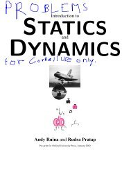
<strong>Introduction</strong> <strong>to</strong><br />
STATICS<br />
<strong>and</strong><br />
DYNAMICS<br />
<strong>Andy</strong> <strong>Ruina</strong> <strong>and</strong> <strong>Rudra</strong> <strong>Pratap</strong><br />
c <strong>Rudra</strong> <strong>Pratap</strong> <strong>and</strong> <strong>Andy</strong> <strong>Ruina</strong>, 1994-2008. All rights reserved. No part of this book may be reproduced, s<strong>to</strong>red in a<br />
retrieval system, or transmitted, in any form or by any means, electronic, mechanical, pho<strong>to</strong>copying, or otherwise, without<br />
prior written permission of the authors.<br />
This book is a pre-release version of a book in progress for Oxford University Press.<br />
Acknowledgements. The following are amongst those who have helped with this book as edi<strong>to</strong>rs, artists, tex programmers,<br />
advisors, critics or sugges<strong>to</strong>rs <strong>and</strong> crea<strong>to</strong>rs of content: William Adams, Alexa Barnes, Joseph Burns, Jason Cortell,<br />
Gabor Domokos, Max Donelan, Thu Dong, Gail Fish, Mike Fox, John Gibson, Robert Ghrist, Saptarsi Haldar, Dave Heimstra,<br />
Theresa Howley, Herbert Hui, Michael Marder, Elaina McCartney, Horst Nowacki, Kalpana <strong>Pratap</strong>, Richard R<strong>and</strong>,<br />
Dane Quinn, C.V. Radakrishnan, Phoebus Rosakis, Les Schaeffer, Ishan Sharma, David Shipman, Jill Startzell, Saskya van<br />
Nouhuys, Tian Tang, Kim Turner <strong>and</strong> Bill Zobrist. We certify Arthur Ogawa, Ivan Dobrianov, <strong>and</strong> Stephen Hicks as TeX<br />
geniuses. Mike Coleman worked extensively on the text, wrote many of the examples <strong>and</strong> homework problems <strong>and</strong> made<br />
many figures. David Ho, R. Manjula <strong>and</strong> Abhay drew or improved most of the drawings. Credit for some of the homework<br />
problems retrieved from Cornell archives is due <strong>to</strong> various Theoretical <strong>and</strong> Applied Mechanics faculty. Harry Soodak <strong>and</strong><br />
Martin Tiersten provided some problems from their incomplete book. Our on-again off-again edi<strong>to</strong>r Peter Gordon has been<br />
supportive throughout. Many other friends, colleagues, relatives, students, <strong>and</strong> anonymous reviewers have also made helpful<br />
suggestions.<br />
Software we have used <strong>to</strong> prepare this book includes TEXshop (for L A TEX), Adobe Illustra<strong>to</strong>r, GraphicsConverter <strong>and</strong> MAT-<br />
LAB.
Brief Contents<br />
Front tables . . . . . . . . . . . . . . . . . . . . . . . . . . . . . . . i<br />
Brief Contents . . . . . . . . . . . . . . . . . . . . . . . . . . . . . . 1<br />
Detailed Contents . . . . . . . . . . . . . . . . . . . . . . . . . . . . 2<br />
Preface . . . . . . . . . . . . . . . . . . . . . . . . . . . . . . . . . . 10<br />
Part I: Basics for Mechanics 22<br />
1 What is mechanics . . . . . . . . . . . . . . . . . . . . . . . . . 22<br />
2 Vec<strong>to</strong>rs . . . . . . . . . . . . . . . . . . . . . . . . . . . . . . . 36<br />
3 FBDs . . . . . . . . . . . . . . . . . . . . . . . . . . . . . . . . 140<br />
Part II: Statics 178<br />
4 Statics of one object . . . . . . . . . . . . . . . . . . . . . . . . . 178<br />
5 Trusses <strong>and</strong> frames . . . . . . . . . . . . . . . . . . . . . . . . . 246<br />
6 Transmissions <strong>and</strong> mechanisms . . . . . . . . . . . . . . . . . . . 308<br />
7 Hydrostatics . . . . . . . . . . . . . . . . . . . . . . . . . . . . . 360<br />
8 Tension, shear <strong>and</strong> bending moment . . . . . . . . . . . . . . . . 376<br />
Part III: Dynamics 396<br />
9 Dynamics in 1D . . . . . . . . . . . . . . . . . . . . . . . . . . . 396<br />
10 Particles in space . . . . . . . . . . . . . . . . . . . . . . . . . . 514<br />
11 Many particles in space . . . . . . . . . . . . . . . . . . . . . . . 562<br />
12 Straight line motion . . . . . . . . . . . . . . . . . . . . . . . . . 588<br />
13 Circular motion . . . . . . . . . . . . . . . . . . . . . . . . . . . 626<br />
14 Planar motion of an object . . . . . . . . . . . . . . . . . . . . . 734<br />
15 Kinematics using time-varying basis vec<strong>to</strong>rs . . . . . . . . . . . . 820<br />
16 Constrained particles <strong>and</strong> rigid objects . . . . . . . . . . . . . . . 888<br />
Appendices 956<br />
A Units & Center of mass theorems . . . . . . . . . . . . . . . . . . 956<br />
Answers <strong>to</strong> some homework problems . . . . . . . . . . . . . . . . . 976<br />
Index . . . . . . . . . . . . . . . . . . . . . . . . . . . . . . . . . . 984<br />
Back tables . . . . . . . . . . . . . . . . . . . . . . . . . . . . . . . 989<br />
1
Detailed Contents<br />
Front tables<br />
i<br />
Summary of mechanics . . . . . . . . . . . . . . . . . . . i<br />
Some basic definitions . . . . . . . . . . . . . . . . . . . . ii<br />
Brief Contents 1<br />
Detailed Contents 2<br />
Preface 10<br />
General issues about content, level, organization <strong>and</strong> style, motivation,<br />
how <strong>to</strong> study <strong>and</strong> the use of computers.<br />
0.1 To the student (please read) . . . . . . . . . . . . . . . . . . 14<br />
0.2 A note on computation . . . . . . . . . . . . . . . . . . . . . 18<br />
Box: Informal computer comm<strong>and</strong>s . . . . . . . . . . . . . 21<br />
Part I: Basics for Mechanics 22<br />
1 What is mechanics 22<br />
Mechanics can predict forces <strong>and</strong> motions by using the three pillars of the<br />
subject: I. models of physical behavior, II. geometry, <strong>and</strong> III. the basic<br />
mechanics balance laws. The laws of mechanics are informally summarized<br />
in this introduc<strong>to</strong>ry chapter. The extreme accuracy of New<strong>to</strong>nian<br />
mechanics is emphasized, despite relativity <strong>and</strong> quantum mechanics supposedly<br />
having ‘overthrown’ seventeenth century physics. Various uses<br />
of the word ‘model’ are described.<br />
1.1 The three pillars . . . . . . . . . . . . . . . . . . . . . . . . 23<br />
1.2 Mechanics is wrong, why study it . . . . . . . . . . . . . . 29<br />
1.3 The heirarchy of models . . . . . . . . . . . . . . . . . . . . 31<br />
2 Vec<strong>to</strong>rs 36<br />
The key vec<strong>to</strong>rs for statics, namely relative position, force, <strong>and</strong> moment,<br />
are used <strong>to</strong> motivate needed vec<strong>to</strong>r skills. Notational clarity is emphasized<br />
because correct calculation is impossible without distinguishing<br />
vec<strong>to</strong>rs from scalars. Vec<strong>to</strong>r addition is motivated by the need <strong>to</strong> add<br />
forces <strong>and</strong> relative positions, dot products are motivated as the <strong>to</strong>ol which<br />
reduces vec<strong>to</strong>r equations <strong>to</strong> scalar equations, <strong>and</strong> cross products are motivated<br />
as the formula which correctly calculates the heuristically motivated<br />
quantities of moment <strong>and</strong> moment about an axis.<br />
2
Chapter 0. Detailed Contents Detailed Contents 3<br />
2.1 Notation <strong>and</strong> addition . . . . . . . . . . . . . . . . . . . . . 38<br />
Box 2.1 The scalars in mechanics . . . . . . . . . . . . . . 39<br />
Box 2.2 The Vec<strong>to</strong>rs in Mechanics . . . . . . . . . . . . . 40<br />
2.2 The dot product of two vec<strong>to</strong>rs . . . . . . . . . . . . . . . . 56<br />
Box 2.3 ab cos ) a x b x C a y b y C a z b z . . . . . . . 61<br />
2.3 Cross product <strong>and</strong> moment . . . . . . . . . . . . . . . . . . 65<br />
Box 2.4 Cross product as a matrix multiply . . . . . . . . . 75<br />
Box 2.5 The cross product is distributive over sums . . . . 76<br />
2.4 Solving vec<strong>to</strong>r equations . . . . . . . . . . . . . . . . . . . . 85<br />
Box 2.6 Vec<strong>to</strong>r triangles <strong>and</strong> the laws of sines <strong>and</strong> cosines . 88<br />
Box 2.7 Existence, uniqueness, <strong>and</strong> geometry . . . . . . . 100<br />
2.5 Equivalent force systems . . . . . . . . . . . . . . . . . . . . 105<br />
Box 2.8 means add . . . . . . . . . . . . . . . . . . . . 107<br />
Box 2.9 Equivalent at one point ) equivalent at all points 108<br />
Box 2.10 A “wrench” can represent any force system . . . 109<br />
2.6 Center of mass <strong>and</strong> gravity . . . . . . . . . . . . . . . . . . . 114<br />
Box 2.11 Like , the symbol also means add . . . . . . 115<br />
Box 2.12 Each subsystem is like a particle . . . . . . . . . 119<br />
Box 2.13 The COM of a triangle is at h=3 . . . . . . . . . 123<br />
Problems for Chapter 2 . . . . . . . . . . . . . . . . . . . . . . . 129<br />
3 FBDs 140<br />
A free-body diagram is a sketch of the system <strong>to</strong> which you will apply the<br />
laws of mechanics, <strong>and</strong> all the non-negligible external forces <strong>and</strong> couples<br />
which act on it. The diagram indicates what material is in the system. The<br />
diagram shows what is, <strong>and</strong> what is not, known about the forces. Generally<br />
there is a force or moment component associated with any connection<br />
that causes or prevents a motion. Conversely, there is no force or moment<br />
component associated with motions that are freely allowed. Mechanics<br />
reasoning entirely rests on free body diagrams. Many student errors in<br />
problem solving are due <strong>to</strong> problems with their free body diagrams, so<br />
we give tips about how <strong>to</strong> avoid various common free-body diagram mistakes.<br />
3.1 Interactions, forces & partial FBDs . . . . . . . . . . . . . . 142<br />
Vec<strong>to</strong>r notation for FBDs . . . . . . . . . . . . . . . . . . 145<br />
Box 3.1 Free body diagram first, mechanics reasoning after 152<br />
Box 3.2 Action <strong>and</strong> reaction on partial FBD’s . . . . . . . 154<br />
3.2 Contact: Sliding, friction, <strong>and</strong> rolling . . . . . . . . . . . . . 161<br />
Box 3.3 A problem with the concept of static friction . . . . 165<br />
Box 3.4 A critique of Coulomb friction . . . . . . . . . . . 170<br />
Problems for Chapter 3 . . . . . . . . . . . . . . . . . . . . . . . 174<br />
Part II: Statics 178<br />
4 Statics of one object 178<br />
Equilibrium of one object is defined by the balance of forces <strong>and</strong> moments.<br />
Force balance tells all for a particle. For an extended body mo-
4 Chapter 0. Detailed Contents Detailed Contents<br />
ment balance is also used. There are special shortcuts for bodies with<br />
exactly two or exactly three forces acting. If friction forces are relevant<br />
the possibility of motion needs <strong>to</strong> be taken in<strong>to</strong> account. Many real-world<br />
problems are not statically determinate <strong>and</strong> thus only yield partial solutions,<br />
or full solutions with extra assumptions.<br />
4.1 Static equilibrium of a particle . . . . . . . . . . . . . . . . . 180<br />
Box 4.1 Existence <strong>and</strong> uniqueness . . . . . . . . . . . . . 184<br />
Box 4.2 The simplification of dynamics <strong>to</strong> statics . . . . . . 186<br />
4.2 Equilibrium of one object . . . . . . . . . . . . . . . . . . . 192<br />
Box 4.3 Two-force bodies . . . . . . . . . . . . . . . . . . 197<br />
Box 4.4 Three-force bodies . . . . . . . . . . . . . . . . . 198<br />
Box 4.5 Moment balance about 3 points is sufficient in 2D . 199<br />
4.3 Equilibrium with frictional contact . . . . . . . . . . . . . . 204<br />
Box 4.6 Wheels <strong>and</strong> two force bodies . . . . . . . . . . . . 208<br />
4.4 Internal forces . . . . . . . . . . . . . . . . . . . . . . . . . 218<br />
4.5 3D statics of one part . . . . . . . . . . . . . . . . . . . . . 224<br />
Problems for Chapter 4 . . . . . . . . . . . . . . . . . . . . . . . 233<br />
5 Trusses <strong>and</strong> frames 246<br />
Here we consider collections of parts assembled so as <strong>to</strong> hold something<br />
up or hold something in place. Emphasis is on trusses, assemblies of<br />
bars connected by pins at their ends. Trusses are analyzed by drawing<br />
free body diagrams of the pins or of bigger parts of the truss (method<br />
of sections). Frameworks built with other than two-force bodies are also<br />
analyzed by drawing free body diagrams of parts. Structures can be rigid<br />
or not <strong>and</strong> redundant or not, as can be determined by the collection of<br />
equilibrium equations.<br />
5.1 Method of joints . . . . . . . . . . . . . . . . . . . . . . . . 248<br />
5.2 The method of sections . . . . . . . . . . . . . . . . . . . . 260<br />
5.3 Solving trusses on a computer . . . . . . . . . . . . . . . . . 267<br />
5.4 Frames . . . . . . . . . . . . . . . . . . . . . . . . . . . . . 277<br />
Box 5.1 The ‘method of bars <strong>and</strong> pins’ for trusses . . . . . 280<br />
5.5 3D trusses <strong>and</strong> advanced truss concepts . . . . . . . . . . . . 287<br />
Box 5.2 Stuctural rigidity <strong>and</strong> geometric congruence . . . 293<br />
Box 5.3 Rigidity, redundancy, linear algebra <strong>and</strong> maps . . 294<br />
Problems for Chapter 5 . . . . . . . . . . . . . . . . . . . . . . . 302<br />
6 Transmissions <strong>and</strong> mechanisms 308<br />
Some collections of solid parts are assembled so as <strong>to</strong> cause force or<br />
<strong>to</strong>rque in one place given a different force or <strong>to</strong>rque in another. These<br />
include levers, gear boxes, presses, pliers, clippers, chain drives, <strong>and</strong><br />
crank-drives. Besides solid parts connected by pins, a few specialpurpose<br />
parts are commonly used, including springs <strong>and</strong> gears. Tricks<br />
for amplifying force are usually based on principals idealized by pulleys,<br />
levers, wedges <strong>and</strong> <strong>to</strong>ggles. Force-analysis of transmissions <strong>and</strong><br />
mechanisms is done by drawing free body diagrams of the parts, writing<br />
equilibrium equations for these, <strong>and</strong> solving the equations for desired<br />
unknowns.
Chapter 0. Detailed Contents Detailed Contents 5<br />
6.1 Springs . . . . . . . . . . . . . . . . . . . . . . . . . . . . . 310<br />
Box 6.1 ‘Zero-length’ springs . . . . . . . . . . . . . . . . 311<br />
Box 6.2 A puzzle with two springs <strong>and</strong> three ropes. . . . . . 318<br />
Box 6.3 How stiff a spring is a solid rod . . . . . . . . . . 319<br />
Box 6.4 Stiffer but weaker . . . . . . . . . . . . . . . . . . 319<br />
Box 6.5 2D geometry of spring stretch . . . . . . . . . . . 321<br />
6.2 Force amplification . . . . . . . . . . . . . . . . . . . . . . 330<br />
6.3 Mechanisms . . . . . . . . . . . . . . . . . . . . . . . . . . 340<br />
Box 6.6 Shears with gears . . . . . . . . . . . . . . . . . . 344<br />
Problems for Chapter 6 . . . . . . . . . . . . . . . . . . . . . . . 351<br />
7 Hydrostatics 360<br />
Hydrostatics concerns the equivalent force <strong>and</strong> moment due <strong>to</strong> distributed<br />
pressure on a surface from a still fluid. Pressure increases with depth.<br />
With constant pressure the equivalent force has magnitude = pressure<br />
times area, acting at the centroid. For linearly-varying pressure on a<br />
rectangular plate the equivalent force is the average pressure times the<br />
area acting 2/3 of the way down. The net force acting on a <strong>to</strong>tally submerged<br />
object in a constant density fluid is the displace weight acting at<br />
the centroid.<br />
7.1 Fluid pressure . . . . . . . . . . . . . . . . . . . . . . . . . 361<br />
Box 7.1 Adding forces <strong>to</strong> derive Archimedes’ principle . . . 364<br />
Box 7.2 Pressure depends on position but not on orientation 365<br />
Problems for Chapter 7 . . . . . . . . . . . . . . . . . . . . . . . 373<br />
8 Tension, shear <strong>and</strong> bending moment 376<br />
The ‘internal forces’ tension, shear <strong>and</strong> bending moment can vary from<br />
point <strong>to</strong> point in long narrow objects. Here we introduce the notion of<br />
graphing this variation <strong>and</strong> noting the features of these graphs.<br />
8.1 Arbitrary cuts . . . . . . . . . . . . . . . . . . . . . . . . . 377<br />
Problems for Chapter 8 . . . . . . . . . . . . . . . . . . . . . . . 393<br />
Part III: Dynamics 396<br />
9 Dynamics in 1D 396<br />
The scalar equation F D ma introduces the concepts of motion <strong>and</strong> time<br />
derivatives <strong>to</strong> mechanics. In particular the equations of dynamics are<br />
seen <strong>to</strong> reduce <strong>to</strong> ordinary differential equations, the simplest of which<br />
have memorable analytic solutions. The harder differential equations<br />
need be solved on a computer. We explore various concepts <strong>and</strong> applications<br />
involving momentum, power, work, kinetic <strong>and</strong> potential energies,<br />
oscillations, collisions <strong>and</strong> multi-particle systems.<br />
9.1 Force <strong>and</strong> motion in 1D . . . . . . . . . . . . . . . . . . . . 398<br />
Box 9.1 What do the terms in F D ma mean . . . . . . . 403<br />
Box 9.2 Solutions of the simplest ODEs . . . . . . . . . . . 408<br />
Box 9.3 D’Alembert’s mechanics: beginners beware . . . . 411<br />
9.2 Energy methods in 1D . . . . . . . . . . . . . . . . . . . . . 418
6 Chapter 0. Detailed Contents Detailed Contents<br />
Box 9.4 Particle models for the energetics of locomotion . . 429<br />
9.3 Vibrations: mass, spring <strong>and</strong> dashpot . . . . . . . . . . . . . 436<br />
Box 9.5 A cos.t/ C B sin.t/ D R cos.t / . . . . . 441<br />
Box 9.6 Solution of the damped-oscilla<strong>to</strong>r equations . . . . 447<br />
9.4 Coupled motions in 1D . . . . . . . . . . . . . . . . . . . . 461<br />
Box 9.7 Normal modes: the math <strong>and</strong> the recipe . . . . . . 468<br />
9.5 Collisions in 1D . . . . . . . . . . . . . . . . . . . . . . . . 476<br />
Box 9.8 When equal rods collide the vibrations disappear . 481<br />
9.6 Advanced: forcing & resonance . . . . . . . . . . . . . . . . 485<br />
Box 9.9 A Loudspeaker cone is a forced oscilla<strong>to</strong>r. . . . . . 490<br />
Box 9.10 Solution of the forced oscilla<strong>to</strong>r equation . . . . . 492<br />
Box 9.11 The vocabulary of forced oscillations . . . . . . . 493<br />
Problems for Chapter 9 . . . . . . . . . . . . . . . . . . . . . . . 501<br />
10 Particles in space 514<br />
This chapter is about the vec<strong>to</strong>r equation F<br />
* D m * a for one particle.<br />
Concepts <strong>and</strong> applications include ballistics <strong>and</strong> planetary motion. The<br />
differential equations of motion are set-up in cartesian coordinates <strong>and</strong><br />
integrated either numerically, or for special simple cases, by h<strong>and</strong>. Constraints,<br />
forces from ropes, rods, chains floors, rails <strong>and</strong> guides that can<br />
only be found once one knows the acceleration, are not considered.<br />
Box 10.1 New<strong>to</strong>n’s laws in New<strong>to</strong>nian reference frames . . 516<br />
10.1 Dynamics of a particle in space . . . . . . . . . . . . . . . . 517<br />
Box 10.2 The derivative of a vec<strong>to</strong>r depends on frame . . . 524<br />
10.2 Momentum <strong>and</strong> energy . . . . . . . . . . . . . . . . . . . . 533<br />
Box 10.3 Conservative forces <strong>and</strong> non-conservative forces 539<br />
Box 10.4 Particle theorems for momenta <strong>and</strong> energy . . . . 541<br />
10.3 Central-force motion <strong>and</strong> celestial mechanics . . . . . . . . . 545<br />
Problems for Chapter 10 . . . . . . . . . . . . . . . . . . . . . . . 555<br />
11 Many particles in space 562<br />
This more advanced chapter concerns the motion of two or more particles<br />
in space. We will use * F D m * a for each particle. We will use Cartesian<br />
coordinates only. The start is the set up of “two-body” type problems<br />
which are easily generalized <strong>to</strong> 3 or more particles. The first section concerns<br />
smooth motions due <strong>to</strong> forces from gravity, springs, smoothly applied<br />
forces <strong>and</strong> friction. The second section concerns the sudden change<br />
in velocities when impulsive forces are applied.<br />
11.1 Coupled particle motion . . . . . . . . . . . . . . . . . . . . 564<br />
11.2 particle collisions . . . . . . . . . . . . . . . . . . . . . . . 572<br />
Box 11.1 Effective mass . . . . . . . . . . . . . . . . . . . 574<br />
Box 11.2 Energetics of collisions . . . . . . . . . . . . . . 575<br />
Box 11.3 Coefficient of generation . . . . . . . . . . . . . 578<br />
Box 11.4 A particle collision model of running . . . . . . . 579<br />
Problems for Chapter 11 . . . . . . . . . . . . . . . . . . . . . . . 584<br />
12 Straight line motion 588
Chapter 0. Detailed Contents Detailed Contents 7<br />
Here is an introduction <strong>to</strong> kinematic constraint in its simplest context,<br />
systems that are constrained <strong>to</strong> move without rotation in a straight line.<br />
In one dimension pulley problems provide the main example. Two <strong>and</strong><br />
three dimensional problems are covered, such as finding structural support<br />
forces in accelerating vehicles <strong>and</strong> the slowing or incipient capsize<br />
of a braking car or bicycle. Angular momentum balance is introduced as<br />
a needed <strong>to</strong>ol but without the complexities of rotatioinal kinematics.<br />
12.1 1D motion <strong>and</strong> pulleys . . . . . . . . . . . . . . . . . . . . . 590<br />
12.2 1D motion w/ 2D & 3D forces . . . . . . . . . . . . . . . . . 601<br />
Box 12.1 Calculation of * H =C<br />
<strong>and</strong> P *<br />
H=C . . . . . . . . . . . 603<br />
Problems for Chapter 12 . . . . . . . . . . . . . . . . . . . . . . . 614<br />
13 Circular motion 626<br />
After movement on straight-lines the second important special case of<br />
motion is rotation on a circular path. Polar coordinates <strong>and</strong> base vec<strong>to</strong>rs<br />
are introduced in this simplest possible context. The key new idea is that<br />
not just coordinates, but base vec<strong>to</strong>rs, can change with time. The primary<br />
applications are pendulums, gear trains, <strong>and</strong> rotationally accelerating<br />
mo<strong>to</strong>rs or brakes.<br />
13.1 Circular motion kinematics . . . . . . . . . . . . . . . . . . 628<br />
Box 13.1 The motion quantities . . . . . . . . . . . . . . . 632<br />
13.2 Dynamics of particle circular motion . . . . . . . . . . . . . 639<br />
Box 13.2 Other derivations of the pendulum equation . . . 643<br />
13.3 2D rigid-object rotation . . . . . . . . . . . . . . . . . . . . 650<br />
Box 13.3 Rotation is uniquely defined for a rigid object (2D) 651<br />
13.4 2D rigid-object angular velocity . . . . . . . . . . . . . . . . 658<br />
Box 13.4 The fixed New<strong>to</strong>nian reference frame F . . . . . 659<br />
Box 13.5 Pla<strong>to</strong> on spinning in circles as motion (or not) . . 660<br />
Box 13.6 Acceleration of a point, using * ! . . . . . . . . . 661<br />
Box 13.7 Angular velocity * ! <strong>and</strong> the rotation matrix ŒR . 664<br />
13.5 Polar moment of inertia . . . . . . . . . . . . . . . . . . . . 670<br />
Box 13.9 Some examples of 2-D Moment of Inertia . . . . 674<br />
Box 13.8 The perpendicular <strong>and</strong> parallel axis theorems . . 676<br />
13.6 Dynamics of rigid-object planar circular motion . . . . . . . 681<br />
Box 13.10 Angular momentum <strong>and</strong> power . . . . . . . . . 685<br />
Problems for Chapter 13 . . . . . . . . . . . . . . . . . . . . . . . 712<br />
14 Planar motion of an object 734<br />
The main goal here is <strong>to</strong> generate equations of motion for general planar<br />
motion of a (planar) rigid object that may roll, slide or be in free flight.<br />
Multi-object systems are also considered so long as they do not involve<br />
other kinematic constraints between the bodies. Features of the solution<br />
that can be obtained from analysis are discussed, as are numerical solutions.<br />
14.1 Rigid object kinematics . . . . . . . . . . . . . . . . . . . . 736<br />
14.2 Mechanics of a rigid-object . . . . . . . . . . . . . . . . . . 752<br />
Box 14.1 2-D mechanics makes sense in a 3-D world . . . 758<br />
Box 14.2 The center-of-mass theorems for 2-D rigid bodies 759
8 Chapter 0. Detailed Contents Detailed Contents<br />
Box 14.3 The work of a moving force <strong>and</strong> of a couple . . . 760<br />
Box 14.4 The vec<strong>to</strong>r triple product * A ¢ . * B ¢ * C / . . . . . 761<br />
14.3 Kinematics of rolling <strong>and</strong> sliding . . . . . . . . . . . . . . . 767<br />
Box 14.5 The Sturmey-Archer hub . . . . . . . . . . . . . 770<br />
14.4 Mechanics of contact . . . . . . . . . . . . . . . . . . . . . 780<br />
14.5 Collisions . . . . . . . . . . . . . . . . . . . . . . . . . . . 798<br />
15 Kinematics using time-varying basis vec<strong>to</strong>rs 820<br />
Here is a second take on the kinematics of particle motion but now using<br />
base vec<strong>to</strong>rs which change with time. The discussion of polar coordinates<br />
started in Chapter 13 is completed here. Path coordinates, where one<br />
base vec<strong>to</strong>r is parellel <strong>to</strong> the velocity <strong>and</strong> the others orthogonal <strong>to</strong> that,<br />
are introduced. The challenging <strong>to</strong>pic of kinematics of relative motion<br />
is in two stages: first using rotating base vec<strong>to</strong>rs connected <strong>to</strong> a moving<br />
rigid object <strong>and</strong> then using the more abstract notation associated with<br />
frame-dependent differentiation <strong>and</strong> the famous “five term acceleration<br />
formula.”<br />
15.1 Polar coordinates <strong>and</strong> path coordinates . . . . . . . . . . . . 821<br />
15.2 Rotating frames <strong>and</strong> their base vec<strong>to</strong>rs . . . . . . . . . . . . 836<br />
Box 15.1 The P * Q formula . . . . . . . . . . . . . . . . . . 845<br />
15.3 General formulas for * v <strong>and</strong> * a . . . . . . . . . . . . . . . . . 850<br />
Box 15.2 Moving frames <strong>and</strong> polar coordinates . . . . . . 856<br />
15.4 Kinematics of 2-D mechanisms . . . . . . . . . . . . . . . . 862<br />
15.5 Advanced kinematics of planar motion . . . . . . . . . . . . 875<br />
Box 15.3 Skates, wheels <strong>and</strong> non-holonomic constraints . . 877<br />
16 Constrained particles <strong>and</strong> rigid objects 888<br />
The dynamics of particles <strong>and</strong> rigid bodies is studied using the relativemotion<br />
kinematics ideas from chapter 15. This is the caps<strong>to</strong>ne chapter<br />
for a two-dimensional dynamics course. After this chapter a good student<br />
should be able <strong>to</strong> navigate through <strong>and</strong> use most of the skills in the<br />
concept map inside the back cover.<br />
16.1 Mechanics of a constrained particle . . . . . . . . . . . . . . 890<br />
Box 16.1 Some brachis<strong>to</strong>chrone curiosities . . . . . . . . . 896<br />
16.2 One-degree-of-freedom 2-D mechanisms . . . . . . . . . . . 912<br />
Box 16.2 Ideal constraints <strong>and</strong> workless constraints . . . . 913<br />
Box 16.3 1 DOF systems oscillate at E P minima . . . . . . 918<br />
16.3 Multi-degree-of-freedom 2-D mechanisms . . . . . . . . . . 926<br />
Appendices 956<br />
A Units & Center of mass theorems 956<br />
Some things that are important, but don’t fit in the flow of a homeworkdriven<br />
course.<br />
First, issues related <strong>to</strong> units <strong>and</strong> dimensions, most importantly that a<br />
quantity is the product of a number <strong>and</strong> a unit. Thus units are part of a<br />
calculation. Some simple advice follows: a) balance units, b) carry units<br />
<strong>and</strong> c) check units. Rules for changing units also follow.
Chapter 0. Detailed Contents Detailed Contents 9<br />
Second, the center of mass allows simplifications for expressions for<br />
momentum, angular momentum, <strong>and</strong> kinetic energy. Furthermore, the<br />
energy equations for systems of particles provide foreshadowing for the<br />
first law of thermodynamics.<br />
A.1 Units <strong>and</strong> dimensions . . . . . . . . . . . . . . . . . . . . . 957<br />
Box A.1 Examples of advised <strong>and</strong> ill-advised use of units . 963<br />
Box A.2 Improvement <strong>to</strong> the old h<strong>and</strong>book approach . . . . 964<br />
Box A.3 Force, Weight <strong>and</strong> English Units . . . . . . . . . . 966<br />
A.2 Theorems for Systems . . . . . . . . . . . . . . . . . . . . . 967<br />
Box A.4 Velocity <strong>and</strong> acceleration of the center-of-mass . . 967<br />
Box A.5 Simplifying H * =C<br />
using the center of mass . . . . . 970<br />
*<br />
Box A.6 Relation between d H<br />
dt =C<br />
<strong>and</strong> H * =C<br />
. . . . . . . . . 972<br />
Box A.7 Using H * *<br />
=O<br />
<strong>and</strong> P H=O <strong>to</strong> find H * *<br />
=C<br />
<strong>and</strong> P H=C . . . . . 973<br />
Box A.8 System momentum balance from * F D m * a . . . . . 974<br />
Box A.9 Rigid-object simplifications . . . . . . . . . . . . 975<br />
Answers <strong>to</strong> some homework problems 976<br />
Index 984<br />
Back tables 989<br />
Momenta <strong>and</strong> energy formulas . . . . . . . . . . . . . . . 989<br />
* v <strong>and</strong><br />
* a by various methods . . . . . . . . . . . . . . . . . 990<br />
Moment of inertia: general facts . . . . . . . . . . . . . . 991<br />
Moment of inertia: example objects . . . . . . . . . . . . . 992<br />
Concept map for Dynamics problems . . . . . . . . . . . . 993
10 Chapter 0. Preface Preface<br />
Preface<br />
General issues about content, level, organization <strong>and</strong> style, motivation, how<br />
<strong>to</strong> study <strong>and</strong> the use of computers.<br />
This is an engineering statics <strong>and</strong> dynamics text intended as both an introduction<br />
<strong>and</strong> as a reference. It is aimed primarily at middle-level engineering<br />
students. The book emphasizes use of vec<strong>to</strong>rs, free-body diagrams, momentum<br />
<strong>and</strong> energy balance <strong>and</strong> computation. Intuitive approaches are discussed<br />
throughout.<br />
Prerequisite <strong>and</strong> co-requisite skills.<br />
some skills.<br />
We assume some students start with<br />
Freshman calcululus. Readers are assumed <strong>to</strong> have facility with the<br />
basic geometry, algebra, trigonometry, differentiation <strong>and</strong> integration<br />
used in elementary calculus. Some of these <strong>to</strong>pics are briefly reviewed<br />
in this book, but not as ab initio tu<strong>to</strong>rials.<br />
This books shows how <strong>to</strong> set-up algebraic <strong>and</strong> differential equations for computer<br />
solution using a pseudo-language easily translated in<strong>to</strong> any common<br />
computer language or package.<br />
We assume the student knows or is learning a computer language or<br />
package in which they can solve sets of linear algebraic equations,<br />
make plots <strong>and</strong> numerically integrate simple ordinary differential equations.<br />
Many students will have had exposure <strong>to</strong> other useful subjects detailed foreknowledge<br />
of which this book does not assume.<br />
Completion of freshman physics may help but is not needed.<br />
Vec<strong>to</strong>r <strong>to</strong>pics, especially dot <strong>and</strong> cross products, are introduced here<br />
from scratch in the context of mechanics.<br />
A background in linear algebra wouldn’t hurt, but the reduction of linear<br />
equations <strong>to</strong> matrix form is taught here. A key fact from linear<br />
algebra, also presented here, is that linear algebraic equations are generally<br />
amenable <strong>to</strong> simple computer solution.<br />
A course in differential equations would also add context. But the basic<br />
concepts of differential equations are presented here as needed.
Chapter 0. Preface Preface 11<br />
Organization<br />
Mechanics could be subdivided in<strong>to</strong> statics vs dynamics, particle vs rigid object<br />
vs many objects (‘multi-object’), <strong>and</strong> 1 vs 2 vs 3 spatial dimensions (1D,<br />
2D & 3D). Thus a mechanics table of contents might have one chunk of text<br />
for each of the 2 ¢ 3 ¢ 3 D 18 combinations:<br />
I. Statics<br />
II. Dynamics<br />
A. particle<br />
£ 1D, 2D, 3D<br />
B. rigid object<br />
£ 1D, 2D, 3D<br />
C. many objects<br />
£ 1D, 2D, 3D<br />
A. particle<br />
£ 1D, 2D, 3D<br />
B. rigid object<br />
£ 1D, 2D, 3D<br />
C. many objects<br />
£ 1D, 2D, 3D<br />
However, these 2 ¢ 3 ¢ 3 D 18 chunks vary greatly in difficulty; 1D statics<br />
is low-level high school material <strong>and</strong> 3D multi-object dynamics is difficult<br />
graduate material. Further, the chunks use various overlapping concepts <strong>and</strong><br />
skills. So it is not sensible <strong>to</strong> organize a book in<strong>to</strong> 18 corresponding chapters.<br />
Nonetheless, some vestiges of the scheme above are used in all books, <strong>and</strong><br />
the general flow of this book is from the bot<strong>to</strong>m back left corner of the box in<br />
the figure, <strong>to</strong>wards the diagonal opposite. The details of the organization, as<br />
visible in the annotated table of contents on the previous pages, has evolved<br />
through trial <strong>and</strong> error, review <strong>and</strong> revision, <strong>and</strong> many semesters of student<br />
testing.<br />
The first eight chapters cover the basics of statics <strong>and</strong> the rest of the book<br />
covers the basics of engineering dynamics. Relatively harder <strong>to</strong>pics, which<br />
might be skipped in quicker or less-advanced courses, are identifiable by<br />
chapter, section or subsection titles like “three-dimensional” or “advanced”.<br />
many<br />
bodies<br />
one <br />
body<br />
particle<br />
static<br />
dynamic<br />
complexity<br />
of objects<br />
1D<br />
how much<br />
inertia<br />
2D<br />
number of <br />
spatial<br />
dimensions<br />
3D<br />
Coverage for courses. The sections have been divided so that the homework<br />
problems selected from one section are usually about half of a typical<br />
weekly homework assignment. The theory <strong>and</strong> examples from one section<br />
might be adequately covered in about one lecture, plus or minus.<br />
A leisurely one semester statics course, or a more fast-paced halfsemester<br />
prelude <strong>to</strong> strength of materials should use chapters 1-8, excluding<br />
<strong>to</strong>pics of less interest. A typical one semester dynamics course will cover<br />
most of of chapters 9-16, reviewing chapters 1-3 at the start. A lower-level<br />
one-semester statics <strong>and</strong> dynamics course can cover the less advanced parts<br />
of chapters 1-6 <strong>and</strong> 9-14. An advanced full-year statics <strong>and</strong> dynamics course<br />
could cover most of the book. That is, the statics portion of the book fits<br />
easily in a semester <strong>and</strong> the whole of the dynamics portion in a bit more than<br />
a semester. Chapters 15-16 can also be used as a start for a second advanced<br />
dynamics course. A student who has learned the statics part of this book is<br />
well-prepared for using statics in engineering practice, for learning Strength<br />
of Materials <strong>and</strong> for going on <strong>to</strong> Dynamics. A student who has learned the<br />
dynamics portion is well prepared <strong>to</strong> go on <strong>to</strong> learn Vibrations, Systems Dy-
12 Chapter 0. Preface Preface<br />
namics or more advanced Multi-object Dynamics.<br />
Organization <strong>and</strong> formatting<br />
Each subject is covered in various ways.<br />
Every section starts with descriptive text <strong>and</strong> short examples motivating<br />
<strong>and</strong> describing the theory;<br />
More detailed explanations of the theory are in boxes interspersed in<br />
the text. For example, one box explains the common derivation of angular<br />
momentum balance from * F D m * a (page 974), one explains the<br />
genius of the wheel (page 208), <strong>and</strong> another connects * ! based kinematics<br />
<strong>to</strong> Oe r <strong>and</strong> Oe based kinematics (page 856);<br />
Sample problems (marked with a gray border) at the end of each section<br />
show how <strong>to</strong> do homework-like calculations. These set an example<br />
by their consistent use of free-body diagrams, systematic application<br />
of basic principles, vec<strong>to</strong>r notation, units, <strong>and</strong> checks against both intuition<br />
<strong>and</strong> special cases;<br />
Homework problems at the end of each chapter give students a chance<br />
<strong>to</strong> practice mechanics calculations. The first problems for each section<br />
build a student’s confidence with the basic ideas. The problems are<br />
ranked in approximate order of difficulty, with theoretical problems<br />
coming later. Problems marked with a * have an answer at the back<br />
of the book;<br />
Reference tables on the inside covers <strong>and</strong> end pages concisely summarize<br />
much of the content in the book. These tables can save students<br />
the time of hunting for formulas <strong>and</strong> definitions.<br />
Notation<br />
Clear vec<strong>to</strong>r notation helps students do problems. One common class of<br />
student errors comes from copying a textbook’s printed bold vec<strong>to</strong>r F the<br />
same way as a plain-text scalar F . We reduce this error by use a redundant<br />
vec<strong>to</strong>r notation, a bold <strong>and</strong> harpooned F * .<br />
As for all authors <strong>and</strong> teachers concerned with motion in two <strong>and</strong> three<br />
dimensions we have struggled with the tradeoffs between a precise notation<br />
<strong>and</strong> a simple notation. Perfectly precise notations are complex <strong>and</strong> intimidating.<br />
Simple notations are ambiguous <strong>and</strong> hide key information. Our attempt<br />
at clarity without <strong>to</strong>o-much clutter is summarized in the box on page 40.<br />
1 For example, we use angular<br />
momentum balance (appropriately<br />
expressed) with respect <strong>to</strong> any possiblyaccelerating<br />
point, not just points<br />
selected from an arcane list.<br />
Relation <strong>to</strong> other mechanics books<br />
The bulk of the content of this book can be found in other places including<br />
freshman physics texts, other engineering texts, <strong>and</strong> hundreds of classics.<br />
Nonetheless this book is in some ways different in organization <strong>and</strong> approach.<br />
It also uses some important but not well-enough known concepts 1 .<br />
Mastery of freshman physics (e.g., from Halliday, Resnick & Walker, Tipler,
Chapter 0. Preface Preface 13<br />
or Serway) would encompass some of this book’s contents. However, after<br />
freshman physics students often have only a vague notion of what mechanics<br />
is, <strong>and</strong> how it can be used. For example many students leave freshman<br />
physics with the sense that a free-body diagram (or ‘force diagram’) is a<br />
vague conceptual picture with arrows for various forces <strong>and</strong> motions drawn<br />
on it this way <strong>and</strong> that. Even the freshman-text illustrations sometimes do not<br />
make clear which force is acting on which object. Also, because freshman<br />
physics tends <strong>to</strong> avoid use of college math, many students leave freshman<br />
physics with little sense of how <strong>to</strong> use vec<strong>to</strong>rs or calculus <strong>to</strong> solve mechanics<br />
problems. This book aims <strong>to</strong> lead students who may start with these fuzzy<br />
freshman-physics notions in<strong>to</strong> a world of precise, yet still intuitive, mechanics.<br />
Various statics <strong>and</strong> dynamics textbooks cover much of the same material<br />
as this one. These textbooks have modern applications, ample samples, lots<br />
of pictures, <strong>and</strong> lots of homework problems. Many are excellent in some<br />
ways. Most of <strong>to</strong>day’s engineering professors learned from one of these<br />
books. Nonetheless we wrote this book hoping <strong>to</strong> do still better. Some of<br />
our goals include<br />
showing the unity of the subject,<br />
presenting a complete description of the subject,<br />
clear notation in figures <strong>and</strong> equations,<br />
integration of the applicability of computers,<br />
consistent use of units throughout,<br />
introduction of various insights in<strong>to</strong> how things work,<br />
a friendly writing style.<br />
Between about 1689 <strong>and</strong> 1960 hundreds of books were written with titles<br />
like Statics, Engineering mechanics, Dynamics, Machines, Mechanisms,<br />
Kinematics, or Elementary physics. Many thoughtfully cover most of the<br />
material here <strong>and</strong> sometimes much more. But none are good modern textbooks;<br />
they lack an appropriate pace, style <strong>and</strong> organization; they are <strong>to</strong>o<br />
reliant on geometry skills <strong>and</strong> not enough on vec<strong>to</strong>rs <strong>and</strong> numerics; <strong>and</strong> they<br />
don’t have enough modern applications, samples calculations, illustrations,<br />
or homework problems. But much good mechanics can be found only in<br />
these older books 2 . If you love mechanics you will enjoy pondering ideas<br />
in some of these books.<br />
What do you think<br />
We have tried <strong>to</strong> make it as easy as possible for you <strong>to</strong> learn basic mechanics<br />
from this book. We present truth as we know it <strong>and</strong> as we think it is effectively<br />
communicated. Nonetheless we have surely made some technical <strong>and</strong><br />
strategic errors. Please let us know your thoughts so that we can improve<br />
future editions.<br />
<strong>Rudra</strong> <strong>Pratap</strong>, pratap@mecheng.iisc.ernet.in<br />
<strong>Andy</strong> <strong>Ruina</strong>,<br />
ruina@cornell.edu<br />
2 Here are three good <strong>and</strong> universally<br />
respected classics:<br />
J.P. Den Har<strong>to</strong>g’s Mechanics originally<br />
published in 1948 but still<br />
available as an inexpensive reprint (well<br />
written <strong>and</strong> insightful);<br />
J.L. Synge <strong>and</strong> B.A. Griffith, Principles<br />
of Mechanics through page 408. Originally<br />
published in 1942, reprinted in<br />
1959 (good pedagogy but dry); <strong>and</strong><br />
E.J. Routh’s, Dynamics of a System<br />
of rigid bodies, Vol 1 (the<br />
“elementary” part through chapter 7.<br />
Originally published in 1905, but<br />
reprinted in 1960). Routh also has 5<br />
other idea- packed statics <strong>and</strong> dynamics<br />
books. Routh shared college graduation<br />
honors with the now-more-famous<br />
physicist James Clerk Maxwell.
14 Chapter 0. Preface 0.1. To the student (please read)<br />
0.1 To the student (please read)<br />
Nature’s rules are so strict that, <strong>to</strong> the extent that you know the rules, you can<br />
make reliable predictions about how Nature, the set of all things, behave. In<br />
particular, most objects of concern <strong>to</strong> engineers obediently follow a subset of<br />
Nature’s rules called the laws of New<strong>to</strong>nian mechanics. So, if you learn the<br />
laws of mechanics, as this book should help you <strong>to</strong> do, you will be able <strong>to</strong><br />
make quantitative predictions about how things st<strong>and</strong>, move, <strong>and</strong> fall. And<br />
you will gain intuition about the mechanics part of Nature’s rules.<br />
How <strong>to</strong> use this book<br />
Here is some general guidance.<br />
1 “Exams are harder than homework.”<br />
Some struggling students say “I<br />
can do the homework problems. I just<br />
can’t do the exams. Exams are harder<br />
<strong>and</strong> trickier.” These students may be<br />
fooling themselves. Most exams are not<br />
trickier than the homework. And when<br />
we have checked, many students who<br />
got through homework with help, can’t<br />
do simplified versions of those same<br />
problems when they have no help.<br />
Check your own underst<strong>and</strong>ing<br />
Most likely you want a decent grade by successfully getting through the<br />
homework assignements <strong>and</strong> exams. You will naturally get help by looking<br />
at examples <strong>and</strong> samples in the text or lecture notes, by looking up formulas<br />
in the front <strong>and</strong> back covers of this book, <strong>and</strong> by asking questions of friends,<br />
teaching assistants <strong>and</strong> professors. What good are books, notes, classmates<br />
or teachers if they don’t help you do the homework All the examples <strong>and</strong><br />
sample problems in this book, for example, are just for this purpose.<br />
But watch out. Too-much use of help from books, notes <strong>and</strong> people can<br />
lead <strong>to</strong> self deception 1 . After you have got through a problem using such<br />
help you should, at least sometimes, check that you have actually learned <strong>to</strong><br />
solve the problem.<br />
To see if you have learned <strong>to</strong> do a problem, do it again, justifying each<br />
step, without looking up even one small (‘oh, I almost knew that’) thing.<br />
If you can’t do this, you gain two learning opportunities. First, you can learn<br />
the missing skill or idea. But more deeply, by getting stuck after you have<br />
been able <strong>to</strong> get through with help, you can learn things about your learning<br />
process. Often the real source of difficulty isn’t a key formula or fact, but<br />
something more subtle. Some useful more subtle ideas might be explained<br />
in the general text discussions.<br />
Read the parts that are at your level<br />
You might be science <strong>and</strong> math school-smart, mechanically inclined, or are<br />
especially motivated <strong>to</strong> learn mechanics. Or you might be reluctantly taking<br />
this class <strong>to</strong> fulfil a requirement. In either case this book is meant for you.<br />
The sections start with generally accessible introduc<strong>to</strong>ry material <strong>and</strong> include<br />
simple examples. The early sample problems in each section are also easy.<br />
But we also have discussions of the theory <strong>and</strong> other more advanced applications<br />
<strong>and</strong> asides <strong>to</strong> challenge more motivated students. If you are a nerd,
Chapter 0. Preface 0.1. To the student (please read) 15<br />
please be patient with the slow introductions <strong>and</strong> the calculations that go line<br />
by line without skipping steps. On the other h<strong>and</strong>, if you are just trying <strong>to</strong><br />
get through this course you need not s<strong>to</strong>p <strong>and</strong> admire every side discussion<br />
about his<strong>to</strong>ry or theory.<br />
Calculation strategies <strong>and</strong> skills<br />
We try <strong>to</strong> demonstrate a systematic approach <strong>to</strong> solving problems. But its<br />
impossible <strong>to</strong> reduce all mechanics problem solutions <strong>to</strong> one clear recipe (despite<br />
the generally applicable recipe on the inside back cover). If a precise<br />
recipe existed then someone could write a computer program that followed<br />
it, <strong>and</strong> we would not have written this textbook. Your mind could be freed<br />
from mechanics problem solutions like a calcula<strong>to</strong>r frees you from the tedium<br />
of long division. But there is an art <strong>to</strong> solving mechanics problems <strong>and</strong><br />
underst<strong>and</strong>ing their solutions. This applies <strong>to</strong> homework problems <strong>and</strong> also<br />
engineering design problems. Art <strong>and</strong> human insight, as opposed <strong>to</strong> precise<br />
algorithm or recipe, is what makes engineering require humans <strong>and</strong> not just<br />
computers 2 . We will try <strong>to</strong> teach you some of this art. For starters, here are<br />
some tips.<br />
Underst<strong>and</strong> the question<br />
It is tempting <strong>to</strong> start writing equations <strong>and</strong> quoting principles when you first<br />
see a problem. However, it is usually worth a few minutes (<strong>and</strong> sometimes<br />
a few hours) <strong>to</strong> try <strong>to</strong> get an intuitive sense of a problem before jumping <strong>to</strong><br />
equations. Before you draw any sketches or write equations, think: does the<br />
problem make sense What information has been given What are you trying<br />
<strong>to</strong> find Is what you are trying <strong>to</strong> find determined by what is given What<br />
physical laws make the problem solvable What extra information do you<br />
think you need What information have you been given that you don’t need<br />
You should first get a general sense of the problem <strong>to</strong> steer you through the<br />
technical details.<br />
Some students find they can read every line of sample problems yet cannot<br />
do test problems, or, later on, cannot do applied design work effectively.<br />
This failing may come from following details without spending time, thinking<br />
<strong>and</strong> gaining an overall sense of the problems.<br />
Think through your solution strategy<br />
For problem solutions you read, like those in this book, someone had <strong>to</strong> think<br />
about the order of work. You also have <strong>to</strong> think about the order of your work.<br />
You will find some tips in the text <strong>and</strong> samples. But it is your job <strong>to</strong> own the<br />
material, <strong>to</strong> learn how <strong>to</strong> think about it your own way, <strong>to</strong> become an expert in<br />
your own style, <strong>and</strong> <strong>to</strong> do the work in the way that makes things most clear<br />
<strong>to</strong> you <strong>and</strong> your readers.<br />
2 Computers can do dynamics. To be<br />
honest, this book presents some methods<br />
which computers can h<strong>and</strong>le. Once<br />
a problem has been reduced <strong>to</strong> a precise<br />
mechanical model a computer code<br />
could take over. Say a finite-element<br />
program or a rigid-body dynamics program.<br />
But you will do better at mechanics,<br />
even with a computers help, if<br />
you can do simple mechanics problems<br />
without a computer.<br />
Analogy with long-division. Since<br />
about 1975 division by a 3 (or more)<br />
digit number is done by calcula<strong>to</strong>rs,<br />
not pencil-<strong>and</strong>-paper long-division. But<br />
competence at division without a calcula<strong>to</strong>r,<br />
at least at division by one digit<br />
numbers, allows one <strong>to</strong> quickly catch<br />
calcula<strong>to</strong>r-entry errors. And knowledge<br />
about division (that, for example, its inverse<br />
multiplication, or that division by<br />
zero is bad) is useful. And such knowledge<br />
comes better by practice with numbers<br />
manipulated in one’s head <strong>and</strong> on<br />
paper than just on a calcula<strong>to</strong>r. Similarly<br />
it is useful <strong>to</strong> know mechanicsproblem<br />
methods well, even if some of<br />
those problems can be solved with by a<br />
computer package.
16 Chapter 0. Preface 0.1. To the student (please read)<br />
3 A tree analogy. Energy gets s<strong>to</strong>red<br />
in the roots of a tree. It gets there from<br />
the trunk. The branches feed the trunk,<br />
the twigs feed the branches, <strong>and</strong> the<br />
leaves feed the twigs with energy from<br />
the sun. But the flow goes the opposite<br />
way, from the leaves on down <strong>to</strong> the<br />
roots. But if you try <strong>to</strong> invent a tree by<br />
starting at the leaves with no knowledge<br />
of the root you could easily get lost <strong>and</strong><br />
connect leaves <strong>to</strong> electric wires or gas<br />
pipes — all nonsense. There’s no point<br />
in connecting the leaves <strong>to</strong> anything until<br />
you have a sense of the whole tree.<br />
The order of calculation is often backwards from the order of<br />
thinking<br />
When working out how <strong>to</strong> solve a problem you often start with general principles,<br />
then look at terms you need <strong>to</strong> know. If these are not given, you think<br />
how <strong>to</strong> figure those from other terms <strong>and</strong> so on. On the other h<strong>and</strong>, when you<br />
go <strong>to</strong> calculate an answer you have <strong>to</strong> start with the information given <strong>and</strong><br />
work your way backwards in<strong>to</strong> the equation which has your answer 3 . To<br />
find the net worth of a corporation you add the value of the various divisions.<br />
To get the value of a division you add up the values of the fac<strong>to</strong>ries. For each<br />
fac<strong>to</strong>ry you add up the value of the pieces of machinery. But <strong>to</strong> get an actual<br />
corporate value you have <strong>to</strong> start by evaluating the pieces of machinery<br />
in each fac<strong>to</strong>ry <strong>and</strong> working back up from the known <strong>to</strong>wards the answer.<br />
Beware that<br />
When you read the minimal write-up of a calculation, especially an<br />
algorithmic recipe or computer program, you often are reading in the<br />
inverse order of the thinking that went in <strong>to</strong> generating the solution.<br />
Of course real problem solving goes both ways. You think about what you<br />
need in order <strong>to</strong> calculate what you want. But you also think about what you<br />
can calculate easily from what is given plainly <strong>to</strong> you. You reach from the<br />
broad <strong>to</strong>wards the details. And you work with known details <strong>to</strong>wards answers<br />
of any kind, wanted or not. And you thus hunt out, building from details <strong>and</strong><br />
simultaneously reaching back from the goal, a route leading all the way from<br />
the details <strong>to</strong> the goal.<br />
Look for equations containing unkowns, not for formulas that<br />
evaluate unknowns<br />
In elementary science <strong>and</strong> math we often learn formulas like<br />
V D LW H; d D 1 2 at 2 ; <strong>and</strong> x D b ¦ p b 2 4ac<br />
2a<br />
<strong>to</strong> find V; d; or x. So it is common wishful thinking for newcomers <strong>to</strong> hope<br />
for a formula that generates the sought unknown in terms of given quantities.<br />
Rather, you should<br />
Find relations that contain variables of interest; don’t worry about<br />
whether they are on the right or left side of an equation. Don’t worry<br />
about whether the variables are alone or isolated.<br />
Most often, you will not know a formula where the thing you want is on the<br />
left <strong>and</strong> everything given is on the right. You will have, say,<br />
V D LW H when you want <strong>to</strong> find W from V; L; <strong>and</strong> H ,
Backspace CE C<br />
Chapter 0. Preface 0.1. To the student (please read) 17<br />
d D 1 2 at 2 when you want <strong>to</strong> find t from a <strong>and</strong> d, <strong>and</strong><br />
ax 2 C bx C c D 0 when you want <strong>to</strong> find x from a; b; <strong>and</strong> c.<br />
Once you have got this far the only problem is math 4 . Here are two tricks<br />
of the mind<br />
1) You know a math <strong>and</strong> computer genius. She is helpful but doesn’t<br />
know any mechanics. Make your first task writing things down so she<br />
could finish up for you. She doesn’t want <strong>to</strong> help Then realize that<br />
finishing up without her is a separate job for you. You will do this later<br />
when you wear your math-genius cap.<br />
2) Be an egotist. Pretend you are omniscient <strong>and</strong> know everything. Then<br />
write down true statements about those things; equations that contain<br />
terms that omniscient-you already know: “If I knew x; y <strong>and</strong> z the<br />
following equation would be true.” Then relax your ego a bit. Count<br />
equations <strong>and</strong> unknowns <strong>to</strong> see if you, or at least your math genius<br />
friend, could solve for the things you previously pretended <strong>to</strong> know.<br />
4 For this <strong>and</strong> other courses, you<br />
should be good at solving math problems<br />
with your pencil <strong>and</strong> with a computer.<br />
But you should distinguish between<br />
the task of setting up a math problem<br />
<strong>and</strong> the solving of the problem.<br />
The solving often takes the bulk of the<br />
time <strong>and</strong> paper, but it’s not where your<br />
thoughts should start. The material that<br />
is new for you in this book is largely<br />
about setting up, rather than solving, the<br />
math problems that arrise in mechanics.<br />
Vec<strong>to</strong>rs <strong>and</strong> free-body diagrams<br />
In the <strong>to</strong>olbox of someone who can solve lots of mechanics problems are two<br />
well-worn <strong>to</strong>ols:<br />
A vec<strong>to</strong>r calcula<strong>to</strong>r that always keeps vec<strong>to</strong>rs <strong>and</strong> scalars distinct, <strong>and</strong><br />
A reliable <strong>and</strong> clear free-body diagram drawing <strong>to</strong>ol.<br />
Because many of the terms in mechanics equations are vec<strong>to</strong>rs, the ability <strong>to</strong><br />
do vec<strong>to</strong>r calculations is essential. Because the concept of an isolated system<br />
is at the core of mechanics, every mechanics practitioner needs the ability <strong>to</strong><br />
draw a good free-body diagram. The second <strong>and</strong> third chapters will help you<br />
build your own set of these two most-important <strong>to</strong>ols.<br />
Outside the books<br />
Guarantee: If you learn <strong>to</strong> do clear correct vec<strong>to</strong>r algebra <strong>and</strong> <strong>to</strong> draw<br />
good free-body diagrams you will do well at mechanics. (Assuming, of<br />
course, that you don’t <strong>to</strong>tally s<strong>to</strong>p studying then <strong>and</strong> there.)<br />
Statics<br />
Engineering<br />
254<br />
Math<br />
The books<br />
Thinking outside the books<br />
We do mechanics because we like mechanics. We hope you will <strong>to</strong>o. It’s fun<br />
<strong>to</strong> puzzle out how things work. Its satisfying <strong>to</strong> do calculations that make<br />
realistic predictions. Mechanics is interesting in its own right <strong>and</strong> it feels<br />
good <strong>to</strong> take pride in new skills. We wrote this book because we want <strong>to</strong> help<br />
you learn the subject if you are interested, <strong>and</strong> get through it if you must.<br />
But we don’t know a straightforward path through your resources (say a path<br />
with 4 straight segments) that really gets you <strong>to</strong> deeper underst<strong>and</strong>ing.<br />
Filename:tfigure-outsidethebooks<br />
Dynamics<br />
Figure 0.1: Thinking outside of the<br />
books. A famous puzzle asks: using<br />
4 contiguous straightline segments connect<br />
all 9 dots that are in a square 3 ¢ 3<br />
array. The only solution has segments<br />
extending outside the “box” of 9 points.<br />
Hence the expression “thinking outside<br />
of the box”.
18 Chapter 0. Preface 0.2. A note on computation<br />
We do know that you need <strong>to</strong> think outside of the confines of your usual<br />
study resources. Like when you are relaxed, away from the pressures of<br />
books, notes, pencils or paper, say when you are walking, showering or lying<br />
down. These are the places where you naturally work out life problems, but<br />
they are good places <strong>to</strong> work out mechanics problems <strong>to</strong>o.<br />
Having an animated mechanics discussion with friends is also good. You<br />
should enjoy your inner nerd socially. Are your friends turned off by techtalk<br />
There are billions of people out there, you should be able <strong>to</strong> find one or<br />
two that like <strong>to</strong> talk shop.<br />
0.2 A note on computation<br />
Mechanics is a physical subject. The concepts in mechanics do not depend<br />
on computers. But mechanics is also a quantitative subject; relevant amounts<br />
(of length, mass, force, moment, time, etc) are described with numbers, <strong>and</strong><br />
relations are described using equations <strong>and</strong> formulas. Computers are very<br />
good with numbers <strong>and</strong> formulas. Thus the modern practice of engineering<br />
mechanics uses computers. The most-needed computer skills for mechanics<br />
are:<br />
solution of simultaneous linear algebraic equations,<br />
plotting, <strong>and</strong><br />
numerical solution of ODEs (Ordinary Differential Equations).<br />
More basically, an engineer also needs the ability <strong>to</strong> routinely evaluate st<strong>and</strong>ard<br />
functions (x 3 , cos 1 , etc.), <strong>to</strong> enter <strong>and</strong> manipulate lists <strong>and</strong> arrays of<br />
numbers, <strong>and</strong> <strong>to</strong> write short programs.<br />
Classical languages, applied packages, <strong>and</strong> simula<strong>to</strong>rs<br />
Programming in st<strong>and</strong>ard languages such as Fortran, Basic, Pascal, C++, or<br />
Java probably take <strong>to</strong>o much time <strong>to</strong> use in solving simple mechanics problems.<br />
Thus an engineer needs <strong>to</strong> learn <strong>to</strong> use one or another widely available<br />
computational package (e.g., MATLAB, O-MATRIX, SCI-LAB, OC-<br />
TAVE, MAPLE, MATHEMATICA, MATHCAD, TKSOLVER, LABVIEW,<br />
etc). We assume that students have learned, or are learning such a package.<br />
Although none of the homework here depends on such, we also encourage<br />
you <strong>to</strong> play with packaged mechanics simula<strong>to</strong>rs (e.g., INVENTOR,<br />
WORKING MODEL, ADAMS, DADS, ODE, etc) for testing <strong>and</strong> building<br />
your intuition.<br />
How we explain computation in this book.<br />
Solving a mechanics problem involves<br />
1. Reducing a physical problem <strong>to</strong> a well posed mathematical problem;<br />
2. Solving the math problem using some combination of pencil <strong>and</strong> paper<br />
<strong>and</strong> numerical computation; <strong>and</strong>
Chapter 0. Preface 0.2. A note on computation 19<br />
3. Giving physical interpretation of the mathematical solution.<br />
This book is primarily about setup (a) <strong>and</strong> interpretation (c), which are rather<br />
the same, no matter what method is used <strong>to</strong> solve the equations. If a problem<br />
requires computation, the exact computer comm<strong>and</strong>s vary from package <strong>to</strong><br />
package. And we don’t know which one you are using. So in this book<br />
we express our computer calculations using an informal pseudo computer<br />
language. For reference, typical comm<strong>and</strong>s are summarized on page 21.<br />
Required computer skills<br />
Here, in a little more detail, are the primary computer skills you need.<br />
Linear algebraic equations. Many mechanics problems are statics or<br />
‘instantaneous mechanics’ problems. These problems involve trying<br />
<strong>to</strong> find some forces or accelerations at a given configuration of a system.<br />
These problems can generally be reduced <strong>to</strong> the solution of linear<br />
algebraic equations of this general type: solve<br />
3 x C 4 y D 8<br />
7 x C p 2 y D 3:5<br />
for x <strong>and</strong> y. In practice the number of variables <strong>and</strong> equations can<br />
be quite large. Some computer packages will let you enter equations<br />
almost as written above. In our pseudo language we would write:<br />
set = { 3*x + 4*y = 8<br />
-7*x + sqrt(2)*y = 3.5 }<br />
solve set for x <strong>and</strong> y<br />
Other packages may require you <strong>to</strong> set up your equations in matrix form<br />
<br />
3 p 4 x 8<br />
D or Az D b<br />
7 2 y 3:5<br />
„ ƒ‚ …<br />
A<br />
„ƒ‚…<br />
z<br />
„ ƒ‚ …<br />
b<br />
which in computer-speak might look something like this:<br />
A = [ 3 4<br />
-7 sqrt(2) ]<br />
b = [ 8 3.5 ]’<br />
solve A*z=b for z<br />
where A is a 2 ¢ 2 matrix, b is a column of 2 numbers (the ’ indicates<br />
that the row of numbers b should be transposed in<strong>to</strong> a column), <strong>and</strong><br />
the two elements of z are x <strong>and</strong> y. For systems of two equations, like<br />
above, a computer is hardly needed. But for systems of three equations<br />
pencil <strong>and</strong> paper work is sometimes error prone. Given the tedium,<br />
the propensity for error, <strong>and</strong> the availability of electronic alternatives,<br />
pencil <strong>and</strong> paper solution of four or more equations is an anachronism.<br />
Plotting. In order <strong>to</strong> see how a result depends on a parameter, or <strong>to</strong> see<br />
how a quantity varies with position or time, it is useful <strong>to</strong> see a plot.<br />
Any plot based on more than a few data points or a complex formula is
20 Chapter 0. Preface 0.2. A note on computation<br />
far more easily drawn using a computer than by h<strong>and</strong>. Most often you<br />
can organize your data in<strong>to</strong> a set of .x; y/ pairs s<strong>to</strong>red in an x list <strong>and</strong> a<br />
corresponding y list. A simple computer comm<strong>and</strong> will then plot x vs<br />
y. The pseudo-code below, for example, plots a circle using 100 points<br />
npoints = [0 1 2 3 ... 100]<br />
theta = npoints * 2 * pi / 100<br />
x = cos(theta)<br />
y = sin(theta)<br />
plot y vs x<br />
where npoints is the list of numbers from 1 <strong>to</strong> 100, theta is a list<br />
of 100 numbers evenly spaced between 0 <strong>and</strong> 2 <strong>and</strong> x <strong>and</strong> y are lists<br />
of 100 corresponding x; y coordinate points on a circle.<br />
ODEs The result of using the laws of dynamics is often a set of differential<br />
equations which need <strong>to</strong> be solved. A simple example would be:<br />
Find x at t D 5 given that dx<br />
dt<br />
D x <strong>and</strong> that at t D 0, x D 1.<br />
The solution <strong>to</strong> this problem can be found easily enough by h<strong>and</strong> <strong>to</strong><br />
be x.5/ D e 5 . But often the differential equations are just <strong>to</strong>o hard for<br />
pencil <strong>and</strong> paper solution. Fortunately the numerical solution of ordinary<br />
differential equations (ODEs) is already programmed in<strong>to</strong> scientific<br />
<strong>and</strong> engineering computer packages. The simple problem above<br />
is solved with computer code equivalent <strong>to</strong> these informal comm<strong>and</strong>s:<br />
ODES = { xdot = x }<br />
ICS = { xzero = 1 }<br />
solve ODES with ICS until t=5<br />
which will yield a list of values for paired values for t <strong>and</strong> x the last of<br />
which will be t D 5 <strong>and</strong> x close <strong>to</strong> e 5 148:4.
Chapter 0. Preface 0.2. A note on computation 21<br />
Examples of informal computer comm<strong>and</strong>s<br />
In this book computer comm<strong>and</strong>s are given informally using comm<strong>and</strong>s<br />
that are not as strict as any real computer package. You will<br />
need <strong>to</strong> translate the informal comm<strong>and</strong>s below in<strong>to</strong> comm<strong>and</strong>s your<br />
package underst<strong>and</strong>s. This reference table uses mathematical ideas<br />
which you may or may not know before you read this book, but these<br />
are introduced in the text when needed.<br />
. . . . . . . . . . . . . . . . . . . . . . . . . . . . . . . . . . . . . . . . . . . . . . . . . . . . . . . . . . . . .<br />
x=7 Set the variable x <strong>to</strong> 7.<br />
. . . . . . . . . . . . . . . . . . . . . . . . . . . . . . . . . . . . . . . . . . . . . . . . . . . . . . . . . . . . .<br />
omega=13 Set ! <strong>to</strong> 13.<br />
. . . . . . . . . . . . . . . . . . . . . . . . . . . . . . . . . . . . . . . . . . . . . . . . . . . . . . . . . . . . .<br />
u=[1 0 -1 0]<br />
Define u <strong>and</strong> v <strong>to</strong> be the lists<br />
v=[2 3 4 pi]<br />
shown.<br />
. . . . . . . . . . . . . . . . . . . . . . . . . . . . . . . . . . . . . . . . . . . . . . . . . . . . . . . . . . . . .<br />
t= [.1 .2 .3 ... 5] Set t <strong>to</strong> the list of 50 numbers<br />
implied by the expression.<br />
. . . . . . . . . . . . . . . . . . . . . . . . . . . . . . . . . . . . . . . . . . . . . . . . . . . . . . . . . . . . .<br />
y=v(3)<br />
sets y <strong>to</strong> the third value of v (in<br />
this case 4).<br />
. . . . . . . . . . . . . . . . . . . . . . . . . . . . . . . . . . . . . . . . . . . . . . . . . . . . . . . . . . . . .<br />
A=[1 2 3 6.9<br />
Set A <strong>to</strong> the array shown.<br />
5 0 1 12 ]<br />
. . . . . . . . . . . . . . . . . . . . . . . . . . . . . . . . . . . . . . . . . . . . . . . . . . . . . . . . . . . . .<br />
z= A(2,3) Set z <strong>to</strong> the element of A in the<br />
second row <strong>and</strong> third column.<br />
. . . . . . . . . . . . . . . . . . . . . . . . . . . . . . . . . . . . . . . . . . . . . . . . . . . . . . . . . . . . .<br />
w=[3<br />
Define w <strong>to</strong> be a column vec<strong>to</strong>r.<br />
4<br />
2<br />
5]<br />
. . . . . . . . . . . . . . . . . . . . . . . . . . . . . . . . . . . . . . . . . . . . . . . . . . . . . . . . . . . . .<br />
w = [3 4 2 5]’<br />
Same as above. ’ means<br />
transpose.<br />
. . . . . . . . . . . . . . . . . . . . . . . . . . . . . . . . . . . . . . . . . . . . . . . . . . . . . . . . . . . . .<br />
u+v<br />
Vec<strong>to</strong>r addition. In this case the<br />
result is Œ3 3 3 .<br />
. . . . . . . . . . . . . . . . . . . . . . . . . . . . . . . . . . . . . . . . . . . . . . . . . . . . . . . . . . . . .<br />
u*v<br />
Element by element<br />
multiplication, in this case<br />
Œ2 0 4 0 .<br />
. . . . . . . . . . . . . . . . . . . . . . . . . . . . . . . . . . . . . . . . . . . . . . . . . . . . . . . . . . . . .<br />
sum(w)<br />
Add the elements of w, in this<br />
case 14.<br />
. . . . . . . . . . . . . . . . . . . . . . . . . . . . . . . . . . . . . . . . . . . . . . . . . . . . . . . . . . . . .<br />
cos(w)<br />
Make a new list, each element of<br />
which is the cosine of the<br />
corresponding element of Œw .<br />
. . . . . . . . . . . . . . . . . . . . . . . . . . . . . . . . . . . . . . . . . . . . . . . . . . . . . . . . . . . . .<br />
mag(u)<br />
The square root of the sum of the<br />
squares of the elements in Œu , in<br />
this case 1.41421...<br />
. . . . . . . . . . . . . . . . . . . . . . . . . . . . . . . . . . . . . . . . . . . . . . . . . . . . . . . . . . . . .<br />
u dot v<br />
The vec<strong>to</strong>r dot product of<br />
component lists Œu <strong>and</strong> Œv , (we<br />
could also write sum(A*B).<br />
. . . . . . . . . . . . . . . . . . . . . . . . . . . . . . . . . . . . . . . . . . . . . . . . . . . . . . . . . . . . .<br />
C cross D<br />
The vec<strong>to</strong>r cross product of C<br />
*<br />
<strong>and</strong> D, * assuming the three<br />
element component lists for ŒC<br />
<strong>and</strong> ŒD have been defined.<br />
. . . . . . . . . . . . . . . . . . . . . . . . . . . . . . . . . . . . . . . . . . . . . . . . . . . . . . . . . . . . .<br />
A matmult w<br />
Use the rules of matrix<br />
multiplication <strong>to</strong> multiply ŒA<br />
<strong>and</strong> Œw .<br />
. . . . . . . . . . . . . . . . . . . . . . . . . . . . . . . . . . . . . . . . . . . . . . . . . . . . . . . . . . . . .<br />
eqset = f3x + 2y = 6 Define ‘eqset’ <strong>to</strong> st<strong>and</strong> for the set<br />
6x + 7y = 8g of 2 equations in braces.<br />
. . . . . . . . . . . . . . . . . . . . . . . . . . . . . . . . . . . . . . . . . . . . . . . . . . . . . . . . . . . . .<br />
solve eqset<br />
Solve the equations in ‘eqset’ for<br />
for x <strong>and</strong> y x <strong>and</strong> y.<br />
. . . . . . . . . . . . . . . . . . . . . . . . . . . . . . . . . . . . . . . . . . . . . . . . . . . . . . . . . . . . .<br />
solve Ax=b for x Solve the matrix equation<br />
ŒA Œx D Œb for the list of<br />
numbers x. This assumes A <strong>and</strong><br />
b have already been defined.<br />
. . . . . . . . . . . . . . . . . . . . . . . . . . . . . . . . . . . . . . . . . . . . . . . . . . . . . . . . . . . . .<br />
for i = 1 <strong>to</strong> N<br />
Execute the comm<strong>and</strong>s ‘such <strong>and</strong><br />
such <strong>and</strong> such such’ N times, the first time with<br />
end<br />
i D 1, the second with i D 2, etc<br />
. . . . . . . . . . . . . . . . . . . . . . . . . . . . . . . . . . . . . . . . . . . . . . . . . . . . . . . . . . . . .<br />
plot y vs x<br />
Assuming x <strong>and</strong> y are two lists<br />
of numbers of the same length,<br />
plot the y values vs the x values.<br />
. . . . . . . . . . . . . . . . . . . . . . . . . . . . . . . . . . . . . . . . . . . . . . . . . . . . . . . . . . . . .<br />
solve ODEs<br />
Assuming a set of ODEs <strong>and</strong> ICs<br />
with ICs<br />
until t=5<br />
have been defined, use numerical<br />
integration <strong>to</strong> solve them <strong>and</strong><br />
evaluate the result at t D 5.<br />
. . . . . . . . . . . . . . . . . . . . . . . . . . . . . . . . . . . . . . . . . . . . . . . . . . . . . . . . . . . . .<br />
With an informality consistent with what is written above, other<br />
comm<strong>and</strong>s are introduced as needed.