Introduction to and Andy Ruina and Rudra Pratap

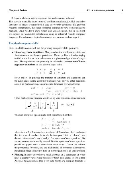
Chapter 0. Preface 0.2. A note on computation 19
3. Giving physical interpretation of the mathematical solution.
This book is primarily about setup (a) and interpretation (c), which are rather
the same, no matter what method is used to solve the equations. If a problem
requires computation, the exact computer commands vary from package to
package. And we don’t know which one you are using. So in this book
we express our computer calculations using an informal pseudo computer
language. For reference, typical commands are summarized on page 21.
Required computer skills
Here, in a little more detail, are the primary computer skills you need.
Linear algebraic equations. Many mechanics problems are statics or
‘instantaneous mechanics’ problems. These problems involve trying
to find some forces or accelerations at a given configuration of a system.
These problems can generally be reduced to the solution of linear
algebraic equations of this general type: solve
3 x C 4 y D 8
7 x C p 2 y D 3:5
for x and y. In practice the number of variables and equations can
be quite large. Some computer packages will let you enter equations
almost as written above. In our pseudo language we would write:
set = { 3*x + 4*y = 8
-7*x + sqrt(2)*y = 3.5 }
solve set for x and y
Other packages may require you to set up your equations in matrix form
3 p 4 x 8
D or Az D b
7 2 y 3:5
„ ƒ‚ …
A
„ƒ‚…
z
„ ƒ‚ …
b
which in computer-speak might look something like this:
A = [ 3 4
-7 sqrt(2) ]
b = [ 8 3.5 ]’
solve A*z=b for z
where A is a 2 ¢ 2 matrix, b is a column of 2 numbers (the ’ indicates
that the row of numbers b should be transposed into a column), and
the two elements of z are x and y. For systems of two equations, like
above, a computer is hardly needed. But for systems of three equations
pencil and paper work is sometimes error prone. Given the tedium,
the propensity for error, and the availability of electronic alternatives,
pencil and paper solution of four or more equations is an anachronism.
Plotting. In order to see how a result depends on a parameter, or to see
how a quantity varies with position or time, it is useful to see a plot.
Any plot based on more than a few data points or a complex formula is