Chapter 9 Viscous flow

Chapter 9
Viscous flow
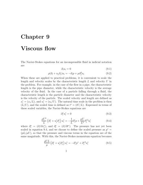
The Navier-Stokes equations for an incompressible fluid in indicial notation
are
∂ i u i = 0 (9.1)
ρ(∂ t + u j ∂ j )u i = −∂ i p + µ∂ 2 j u i (9.2)
When these are applied to practical problems, it is convenient to scale the
length and velocity scales by the characteristic length L and velocity U in
the problem. For example, in the case of the flow in a pipe, the characteristic
length is the pipe diameter, while the characteristic velocity is the average
velocity of the fluid. In the case of a particle falling through a fluid, the
characteristic length is the particle diameter and the characteristic velocity
is the velocity of the particle. The scaled velocity and length are defined as
x ∗ i = (x i /L), and u ∗ i = (u i /U). The natural time scale in the problem is then
(L/U), and the scaled time is defined as t ∗ = (tU/L). Expressed in terms of
these scaled variables, the Navier-Stokes equations are
∂ ∗ i u∗ i = 0 (9.3)
ρU 2 ( )
∂
∗
L t + u ∗ j ∂∗ j u
∗
i = − 1 L ∂∗ i p + µU
L 2 ∂∗ j 2 u ∗ i (9.4)
where ∂i ∗ = (∂/∂x ∗ i ), and ∂∗ t = (∂/∂t ∗ ). The pressure has not yet been
scaled in equation 9.4, and we choose to define the scaled pressure as p ∗ =
(pL/µU), so that the pressure and viscous terms in the equation are of the
same magnitude. With this, the Navier-Stokes momentum equation becomes
ρUL
µ
(
∂
∗
t + u ∗ j∂ ∗ j
)
u
∗
i = −∂ ∗ i p ∗ + ∂ ∗ j 2 u ∗ i (9.5)
1

2 CHAPTER 9. VISCOUS FLOW
The dimensionless number (ρUL/µ) is the Reynolds number, which provides
the ratio of convection and diffusion for the fluid flow. This can also be
written as (UL/ν), where nu = (µ/ρ) is the kinematic viscosity or momentum
diffusivty.
When the Reynolds number is small, the convective terms in the momentum
equation 9.5 can be neglected in comparison to the viscous terms
on the right side of 9.5. The Navier-Stokes equations reduce to the ‘Stokes
equations’ in this limit,
∂ i u i = 0 (9.6)
−∂ i p + µ∂ 2 j u i = 0 (9.7)
The Stokes equations have two important properties — they are linear, since
both the equations are linear in the velocity u i , and they are quasi-steady,
since there are no time derivatives in the Stokes equations. The absence of
time derivatives in the governing equations implies that the velocity field
due to the forces exerted on the fluid depend only on the instanteneous value
of the forces, or the velocity boundary conditions at the surfaces bounding
the fluid, and not the time history of the forces exerted on the fluid. For
example, in order to determine the velocity field due to force exerted by a
sphere falling through a fluid, it is sufficient to know the instanteneous value
of the velocity of the sphere, and it is not necessary to know the details of
the previous evolution of the velocity of the sphere. This is because the flow
is diffusion dominated, and it is assumed that diffusion is instanteneous at
zero Reynolds number. A similar feature is encountered in the solution for
the diffusion equation in the limit of low Peclet number, where convective
effects are neglected.
D∇ 2 c = 0 (9.8)
In this case, the concentration field is determined at any instant if the value
of the boundary conditions at the bounding surfaces are know, and it is not
necessary to know the previous evolution of the previous evolution of the
concentration at the bounding surfaces.
Diffusion is not instanteneous in reality, of course, and there is a distance
beyond which the assumption of instanteneous diffusion is not valid. For
example, consider the case of a sphere settling through a fluid. Though
diffusion is fast compared to convection over lengths comparable to the sphere
diameter in the limit of low Reynolds number, it is expected that there is
some larger length over which diffusion is not instanteneous, and convective

9.1. SPHERICAL HARMONIC SOLUTIONS 3
effects become important. This ‘diffusion length’ L D can be estimated by
balancing the convective and diffusive terms in the momentum equation,
ρu j ∂ j u i ∼ (ρU 2 /L D )
µ∂ 2 j u i ∼ (µU/L D ) (9.9)
A balance between these two indicates that L D ∼ (µ/ρU), or (L D /L) ∼ Re −1 .
Thus, convective effects become important when the ratio of the distance
from the sphere and the sphere radius is large compared to Re −1 .
The linearity of the Stokes equations has some useful consequences. For
example linearity can be used to deduce that if the force exerted by a surface
on a fluid is reversed, then the fluid velocity field is also exactly reversed at
all points in the fluid, as shown in figure 9.1. This is called the ‘Stokes flow
reversibility’. Similarly, if the force exerted by the surfaces on the sphere
is reduced by a factor of 2, then the fluid velocity is also reduced by a
factor of 2 at all points. In addition, linear superposition can be used to
separate a problem into smaller sub-problems, and then add up the results.
For example, consider a sphere moving in a fluid as shown in figure 9.2. This
problem can be separated into three sub-problems, each of which consists
of a sphere which has a velocity along one of the coordinate axes, with the
stipulation that the sum of the three velocity vectors is equal to the velocity
of the sphere in the original problem. The velocity fields in each of these
three sub-problems are calculated, and are added up in order to obtain the
velocity field in the original problem.
9.1 Spherical harmonic solutions
The Stokes equations can be written as two Laplace equations for the pressure
and the velocity fields by taking the divergence of the momentum equation
9.7.
∂ i (−∂ i p + µ∂ 2 j u i)
= −∂ 2 i p + µ∂ 2 j∂ i u i
= −∂ 2 i p (9.10)
Equation 9.10 indicates that the Laplacian of the pressure field is identically
zero,
∂ 2 i p = 0 (9.11)

4 CHAPTER 9. VISCOUS FLOW
x
2
x
2
x
3
x
x
1
x
1
(a)
(b)
Figure 9.1: When the force exerted on the fluid is reversed, the fluid velocity
is reversed at all points in Stokes flow.

9.1. SPHERICAL HARMONIC SOLUTIONS 5
x
2
x
3
x
1
(a)
x
2
x
2
x
2
x
3
x
3
x
1
x1
x1
(b) (c) (d)
Figure 9.2: Use of linear superposition for separating the problem into simpler
sub-problems.

6 CHAPTER 9. VISCOUS FLOW
The velocity field in the momentum equation can be separated into two
parties, a ‘homogeneous solution’ which satisfies
and a particular solution which satisfies
∂ 2 i u (h)
i = 0 (9.12)
µ∂ 2 i u(p) i = ∂ i p (9.13)
The particular solution is any one solution to the equation 9.13. One solution
which satisfies equation 9.13 is
u (p)
i = 1
2µ px i (9.14)
This solution can be verified as follows. If we take the gradient of the particular
solution 9.14, we get
∂ j u (p)
i = 1
2µ (x i∂ j p + pδ ij ) (9.15)
Upon taking the divergence of the above equation, we get
∂j 2 u(p) i = 1
2µ (2δ ij∂ j p + x i ∂j 2 p)
= 1 µ ∂ ip (9.16)
Therefore, the velocity fields can be obtained by solving the Laplace equation
for the pressure and the homogeneous part of the velocity fields, and using
equation 9.16 to obtain the particular part of the velocity field.
We have already studied the solution for the Laplace equation,
∇ 2 φ = 0 (9.17)
which are obtained using separation of variables. In the present chapter, we
derive the same solutions using the more convenient indicial notation. The
fundamental solution for the Laplace equation in three dimensions, correct
to within a multiplicative constant (which is determined from the boundary
conditions, is
Φ (0) = 1 r
(9.18)

9.1. SPHERICAL HARMONIC SOLUTIONS 7
A series of solutions can be derived from equation 9.18 as follows. If we take
the gradient of equation 9.18, we get
∂
∇ 2 φ = ∇ 2 ∂φ = 0 (9.19)
∂x i ∂x i
Therefore, if φ is a solution of the Laplace equation, then its gradient (∂φ/∂x i )
is also a solution of the Laplace equation. The gradient of the fundamental
solution is given by
∂Φ (0)
∂x i
=
(
)
∂ ∂ ∂ 1
e 1 + e 2 + e 3
∂x 1 ∂x 2 ∂x 3 (x 2 1 + x 2 2 + x 2 3) 1/2
= − e 1x 1 + e 2 x 2 + e 3 x 3
(x 2 1 + x 2 2 + x 2 3) 3/2
= − x i
r 3 (9.20)
Therefore, the second solution for the Laplace equation, which is proportional
to the gradient of the first, is
Φ (1)
i
= x i
r 3 (9.21)
The third solution can be obtained by taking the gradient of the second
solution,
Φ (2)
ij
= ∂Φ(1) i
∂x j
= ∂ ( ) xi
∂x j r
(
δij
=
r − 3x )
ix j
r 3
(9.22)
It can easily be verified that the above solutions are linear combinations of
the spherical harmonic solutions obtained by separation of variables. For
example, the three components of Φ (1)
i are
Φ (1)
3 = x 3
r 3

8 CHAPTER 9. VISCOUS FLOW
cos (θ)
=
r 2
= r −2 P1 0 (cos (θ))
Φ (1)
1 = x 1
r 3
sin (θ) cos (φ)
=
r 2
= r −2 P1 1 (cos (θ))((exp (ıφ) + exp (−ıφ))/2
Φ (1)
2 = x 2
=
r 3
sin (θ) sin (φ)
r 2
= r −2 P1 1 (cos (θ))((exp (ıφ) − exp (−ıφ))/(2ı) (9.23)
Similarly, it can be verified that the elements of the second solution Φ (2)
ij are
linear combinations of the second solution obtained from spherical harmonics,
(1/r 3 )P3 m (cos (θ)) exp (ımφ). First note that the tensor Φ (2)
ij is a symmetric
tensor traceless tensor, and the sum of the diagonal elements is identically
equal to zero. Therefore, there are five independent elements in this tensor,
which correspond to the five solutions of the second spherical harmonic for
m = 0, ±1, ±2. The component Φ (2)
Φ (2)
33 =
33 is
( ) 1
r − 3x2 3
3 r 5
= 1 r 3(1 − 3 cos (θ)2 )
= − 2P 3 0 (cos (θ))
(9.24)
r 3
Similarly, the correspondence between the other elements of Φ (2)
ij and the
other spherical harmonic solutions can be shown.
The growing spherical harmonic solutions are obtained by multiplying
the decaying solutions by r 2n+1 , to obtain the series
Φ (0) = 1
= x i
Φ (2) = r 2 δ ij + 3x i x j (9.25)
Φ (1)
The solutions for the homogeneous part of the velocity field and the pressure
field are linear combinations of the growing and decaying solutions.

9.1. SPHERICAL HARMONIC SOLUTIONS 9
9.1.1 Force on a settling sphere
In this section, we use the spherical harmonic expansion in order to determine
for force exerted on a sphere settling in a fluid. The sphere is considered to be
of unit radius, so that all length scales in the problem are scaled by the radius
of the sphere. The sphere has a velocity U, and the boundary conditions at
the surface of the sphere are that the fluid velocity is equal to the velocity
of the sphere,
u i = U i at r = 1 (9.26)
while the velocity decreases to zero at a large distance from the center of the
sphere.
We use a spherical coordinate system, where the origin of the coordinate
system is fixed at the center of the sphere, as shown in figure 9.3. Since the
Stokes equations are linear, the fluid velocity and pressure fields are linear
functions of the velocity U i of the sphere. In addition, the homogeneous
solution for the velocity field and the pressure are solutions of the Laplace
equation, and so these are in the form of spherical harmonics given in 9.18,
9.20, 9.22 and the higher harmonics. The only linear combinations of the
velocity of the sphere U i and the spherical harmonic solutions which can
result in a velocity vector are
(
u (h) 1
i = A 1 U i
r + A δij
2U j
r − 3x )
ix j
3 r 5
(9.27)
where A 1 and A 2 are constants. Similarly, the only linear combinations of
the velocity vector and the spherical harmonic solutions which can result in
the scalar pressure is
p = A 3 U j
x j
r 3 (9.28)
where A 3 is a constant. The total velocity field is the sum of the homogeneous
and particular parts,
(
1
u i = A 1 U i
r + A δij
2U j
r − 3x )
ix j
+ A 3x i U j x j
(9.29)
3 r 5 2µ r 3
The values of the constants A 1 , A 2 and A 3 are determined from the boundary
conditions at the surface of the sphere, 9.26, as well as the incompressibility
condition 9.1 which has not been enforced yet. The incompressibility

10 CHAPTER 9. VISCOUS FLOW
x
3
x 1
x 2
g
U
Figure 9.3: Sphere settling in a fluid.
condition (∂u i /∂x i ) = 0 can be simplified as
∂u i
∂x i
(
∂ 1 ∂
= A 1 U i
∂x i r + A δ ij
2U j
∂x i r − 3 ∂ )
x i x j
+ A 3U j
3 ∂x i r 5 2µ
= − A 1U i x i
r 3 + A 2 U j
(
+ A 3U j
2µ
= − A 1U i x i
r 3
(
δii x j
r 3
+ δ ijx i
r 3
− 3δ ijx i
r 5
− 3δ ijx i
r 5
− 3x2 i x )
j
r 5
− 3δ iix j
r 5
∂ x i x j
∂x i r 3
)
+ 15x2 ix j
r 7
+ A 3U j x j
2µr 3 (9.30)
In simplifying equation 9.30, we have used x 2 i = (x 2 1+x 2 2+x 2 3) = r 2 . Therefore,
from the incompressibility condition, we get A 1 = (A 3 /2µ). Inserting this
into equation 9.30, the velocity field is
(
δij
u i = A 1 U j
r + x ) (
ix j δij
+ A
r 3 2 U j
r − 3x )
ix j
(9.31)
3 r 5
The constants A 1 and A 2 are determined from the boundary condition at the
surface of the sphere (r = 1),
u i | r=1
= A 1 U i + A 1 U j x i x j + A 2 U i − 3A 2 U j x i x j
= U i (9.32)
From this, we get two equations for A 1 and A 2 ,
A 1 + A 2 = 1
A 1 − 3A 2 = 0 (9.33)

9.1. SPHERICAL HARMONIC SOLUTIONS 11
These can be solved to obtain
A 1 = 3 4
A 2 = 1 4
(9.34)
The final solution for the velocity field is
u i = 3U (
j δij
4 r + x )
ix j
+ U j
r 3 4
while the pressure is
(
δij
r − 3x )
ix j
3 r 5
(9.35)
p = 3µU jx j
(9.36)
2r 3
The force exerted on the sphere is given by
∫
F i = dST ik n k
S
∫
= dS(−pn i + τ ik n k ) (9.37)
The shear stress is τ ik = µ((∂u i /∂x k ) + (∂u k /∂x k )). The gradient of the
velocity field, (∂u i /∂x k ), can be determined as follows,
∂u i
= 3U (
j
− δ ijx k
+ δ ikx j
+ δ jkx i
− 3x )
ix j x k
∂x k 4 r 3 r 3 r 3 r 5
+ U (
j
− 3δ ijx k
− 3δ ikx j
− 3δ jkx i
+ 15x )
ix j x k
(9.38)
4 r 5 r 5 r 5 r 7
The gradient (∂u k /∂x i ) is obtained by interchanging the indices i and k in
equation 9.38,
∂u k
= 3U (
j
− δ kjx i
+ δ ikx j
+ δ ijx k
− 3x )
ix j x k
∂x i 4 r 3 r 3 r 3 r 5
+ U (
j
− 3δ jkx i
− 3δ ikx j
− 3δ ijx k
+ 15x )
ix j x k
(9.39)
4 r 5 r 5 r 5 r 7
Adding these two contributions and multiplying by the viscosity, and setting
the radius equal to 1 at the surface of the sphere, we get
( 3Uj
τ ik = µ
2 (δ ikx j − 3x i x j x k )
+ U j
2 (−3δ ijx k − 3δ ik x j − 3δ jk x i + 15x i x j x k )
)
(9.40)

12 CHAPTER 9. VISCOUS FLOW
The unit normal to the surface of the sphere, n i is also equal to the ratio of
the displacement vector and the radius, n i = (x i /r). Since the radius is 1 on
the surface of the sphere, n i = x i . Therefore, the dot product of the stress
tensor and the unit normal is
( 3Uj
τ ik n k = µ
2 (x ix j − 3x i x j x 2 k )
+ U )
j
2 (−3δ ijx 2 k − 6x ix j + 15x i x j x 2 k )
(
= µ − 3U i
2 + 3U )
jx i x j
(9.41)
2
The contribution to the force on the sphere due to the pressure is given by
−pn i | r=1
= − 3µU jx i x j
2
Adding up these two contributions, we get
(9.42)
T ij n j = − 3U i
2
(9.43)
Since the right side of 9.43 is independent of position on the surface of the
sphere, the total force is the product of T ij n j and the surface area of the
sphere, which is 4π for a sphere of unit radius.
F i = 6πµU i (9.44)
For a sphere of radius R, the dependence of the force on the radius is deduced
on the basis of dimensional analysis,
F i = 6πµRU i (9.45)
9.1.2 Effective viscosity of a suspension
A shear flow is applied to a suspension which consists of solid particles with
radius R and volume fraction φ suspended in a fluid of viscosity µ, as shown
in figure 9.4(a). We will assume, for simplicity, that the suspension is dilute,
so that the disturbance to the flow due to one particle does not affect
the surrounding particles. We would like to derive an average constitutive
relation for the suspension of the form
〈T ij 〉 = −〈p〉δ ij + 2µ eff 〈E ij 〉 (9.46)

9.1. SPHERICAL HARMONIC SOLUTIONS 13
(a)
(b)
Figure 9.4: Shear flow of a suspension (a) and the shear flow around a particle
(b).

14 CHAPTER 9. VISCOUS FLOW
where µ eff is the effective viscosity of the suspension, and 〈〉 is a volume
average over the entire volume of the suspension.
The volume averaged symmetric traceless part of the stress tensor can be
expressed as
〈τ ij 〉 = 1 ∫
dV τ ij
V V suspension
⎛
⎞
= 1 ∫
∫
⎝ dV (2µE ij ) + dV (τ ij − 2µE ij ) ⎠
V V suspension
V suspension
= 2µ〈E ij 〉 + 1 ∫
dV (τ ij − 2µE ij ) (9.47)
V V suspension
The second term on the right side of 9.47 is identically equal to zero for the
fluid, from the constitutive equation. Therefore, the second integral reduces
to an integral over the particles,
〈τ ij 〉 = 2µ〈E ij 〉 + 1 ∫
dV (τ ij − 2µE ij ) (9.48)
V V particles
In order to determine the effective viscosity, it is sufficient to consider the
symmetric traceless part of the above equation. Further, if the particles are
solid, the rate of deformation E ij within the particles is identically equal to
zero. Therefore, the symmetric traceless part of the above equation reduces
to
〈τ ij 〉 = 2µ〈E ij 〉 + N ∫
dV (τ ij − 2µE ij ) (9.49)
V V 1 particles
= 2µ〈E ij 〉 + N ∫
dV τ ij (9.50)
V V 1 particle
∫
φ
= 2µ〈E ij 〉 +
dV τ
(4πR 3 ij (9.51)
/3) V 1 particle
In deriving equation 9.51 from 9.50, we have used the simplification that the
number of particles per unit volume is the ratio of the volume fraction and
the volume of a particle. The second term on the right side of equation 9.51
can be simplified as follows. Consider the divergence of (τ il x j ),
∂τ il x j
∂x l
= τ il δ lj + x j
∂τ il
∂x l
(9.52)

9.1. SPHERICAL HARMONIC SOLUTIONS 15
∂τ il
= τ ij + x j
∂x l
(9.53)
= τ ij (9.54)
The divergence of the stress tensor, in the right side of equation 9.53, is zero
if inertial effects are neglected, and therefore, the integral on the right side
of equation 9.51 can be written as
∫
dV τ ij =
V 1 particle
=
∫
dV ∂τ ilx j
V 1 particle
∂x l
∫
dSn l τ il x j (9.55)
S 1 particle
The surface integral on the right side of equation 9.55 can be calculated
using the spherical harmonic expansion, considering a sphere placed in a
linear shear flow in which the fluid velocity at a large distance from the
sphere, u ∞ i = E ij x j . The fluid velocity field at a large distance from the
sphere is given by
and the pressure is
u i = E ij x j
(
)
1 − R5
+ 5x ( )
ix j x k E jk R
5
r 5 2 r − R3
7 r 5
(9.56)
p = 5µR3 x j x k E jk
r 5 (9.57)
Using this, the surface integral on the left side of equation 9.55 can be calculated,
∫
dSn l τ il x j
S 1 particle
With this, we get the effective shear stress
= 20πR3 µE ij
3
〈τ ij 〉 = 2µE ij + 5φµE ij
( )
= 2µ
1 + 5φ 2
(9.58)
E ij (9.59)
Therefore, the effective viscosity is given by µ eff = µ(1 + 5φ/2).

16 CHAPTER 9. VISCOUS FLOW
Exercise: Show that the velocity and pressure fields due to a sphere of
radius R rotating with angular velocity Ω in a fluid which is at rest a large
distance from the sphere is,
u i = ǫ ijk Ω j x k
( R
r
) 3
p = 0 (9.60)
Show that the exerted by the sphere on the fluid is,
L i = −8πµR 3 Ω i (9.61)
Hint: Note that the angular velocity is a pseudo-vector, and the velocity field
and pressure are real.
9.2 Green’s functions and Faxen’s laws:
9.2.1 Oseen tensor for a point force:
Since the Stokes equations are linear equations, it is possible to obtain
Green’s function formulations for the velocity field similar to those obtained
for the temperature field in steady state heat conduction. We briefly revisit
the solution for the conduction equation in chapter , and then we present
the analogous solution for the Stokes equations. In chapter , we solved the
conduction equation,
−k∇ 2 T = Qδ(r − r s ) (9.62)
to obtain the temperature field,
T(r) =
Q
4πK|r − r s |
(9.63)
where r s is the location of the source point. In order to obtain the Green’s
function solution, we first obtained the temperature field for a sphere of
radius R, and then took the limit R → 0 while keeping the heat flux Q finite.
In viscous flows, the equations equivalent of the Green’s function formulation
9.87 are,
∂ i u i = 0 (9.64)
−∂ i p + µ∂ 2 j u i = F i δ(x − x s ) (9.65)
where x s , the location of the force, is the ‘source point’. Note that the right
side of equation 9.90 has dimensions of force per unit volume, since F i is the

9.2. GREEN’S FUNCTIONS AND FAXEN’S LAWS: 17
total force exerted at the point x s , and the delta function has units of inverse
volume.
In order to solve equation 9.89 and 9.90, we can first solve for the velocity
and pressure fields around a spherical particle of finite radius R, and then
take the limit R → 0 while keeping the force F i finite. The solutions for the
velocity and pressure fields were obtained in equations 9.35 and 9.36, and the
force was obtained as a function of the translational velocity of the sphere in
equation 9.44. If we use 9.44 to express the translational velocity in terms of
the force in equations 9.35 and 9.36, we obtain,
u i = F j
8πµ
while the pressure is
(
δij
r + x )
ix j
+ F jR 2
r 3 24π
(
δij
r − 3x )
ix j
3 r 5
(9.66)
p = F jx j
4πr 3 (9.67)
When we take the limit R → 0, the first term on the right in equation 9.91
remains finite while the second becomes negligible, while the term on the
right side of equation 9.92 is finite. Therefore, the velocity and pressure
fields at a field point x due to a point force F i exerted at the source point
x (s) is,
u i = J ij (x − x s )F j (x (s) )
p = K i (x − x (s) )F i (x (s) ) (9.68)
where the ‘Oseen tensors’, J ij and K i , are given by,
J ij (x) = 1 (
δij
8πµ r + x )
ix j
r 3
K i (x) = 1 x i
(9.69)
4π r 3
where r = |x| is the distance from the source point to the field point.
The linearity of the Stokes equations enables us to use superposition to
find the velocity field due to multiple forces. For example, if the are N point
forces F (n)
i located at positions x (n) , where the index n varies from 1 to N,
then the total velocity field is just the superposition of the velocity fields due
to each of these forces,
u i (x) =
N∑
n=1
J ij (x − x (n) )F (n)
j (x (n) )
p(x) = K i (x − x (n) )F i (x (n) ) (9.70)

18 CHAPTER 9. VISCOUS FLOW
Instead of having a discrete set of point forces, if we have a force distribution,
in which the force per unit volume is given by f i (x), the velocity and pressure
fields can be calculated by integrating the appropriate product of the Oseen
tensor and the force distribution over the volume,
∫
u i (x) = dx ′ J ij (x − x ′ )f j (x ′ )
∫
p(x) = dx ′ K i (x − x ′ )F i (x ′ ) (9.71)
9.2.2 Green’s function for force dipoles:
There are often situations where the suspended particles in a fluid a ‘neutrally
buoyant’, so that they exert no net force on the fluid. Examples are for a
solid sphere in a uniform shear flow in equations and , and for a rotating
particle in equations and . The velocity disturbance at a large distance
from the center of the particle decays proportional to r −2 , in contrast to the
decay proportional to r −1 in equation for the flow around a particle which
exerts a net force on the fluid. The far-field velocity can be expressed as a
function of the ‘force dipole moment’, which is defined as the integral over
the sphere of the tensor product of the surface force and the position vector,
∫
Force dipole moment = dSx i f j
∫
= dSx i τ jk n k (9.72)
Note that this definition is analogous to the ‘dipole moment’ for the temperature
field due to a point dipole. The force dipole moment is a second
order tensor, and it is convenient to separate it into a symmetric and an
antisymmetric part. The symmetric part is given by,
S ij = 1 ∫
dS(x i τ jk n k + x j τ ik n k ) (9.73)
2
while the antisymmetric part is,
A ij = 1 2
∫
dS(τ ik n k x j − τ jk n k x i ) (9.74)
The velocity and pressure fields around a point particle which exerts no net
force on the fluid can be expressed in terms of the symmetric and antisymmetric
dipole moments S ij and A ij .

9.2. GREEN’S FUNCTIONS AND FAXEN’S LAWS: 19
In the previous sub-section, we had derived the velocity field due to a
point force by first solving the flow around a sphere of finite radius R, and
then taking the limit R → 0 while keeping the force exerted a constant. The
velocity field due to a force dipole can be obtained by first solving for the
shear flow around a particle for radius R, and taking the limit of the radius
going to zero while keeping the dipole moment fixed. First, we consider the
symmetric dipole moment due to a sphere in a shear flow, for which the
velocity and pressure fields are given by equations and . It can easily
be shown, using symmetry considerations, that the net force exerted by the
sphere on the fluid is identically zero. The symmetric force dipole due to the
sphere is given by,
S ij = 1 ∫
dS(f i x j + x i f j )
2 S
= 1 ∫
dS(τ il n l x j + τ jl n l x i ) (9.75)
2 S
The integrals on the right side of equation were already evaluated in
equation , and the final result for the symmetric force dipole is,
S ij
= 20πµR3 E ij
3
(9.76)
The rate of deformation tensor E ij can be written in terms of the symmetric
force dipole using equation and substituted into equations and for
the velocity and pressure fields.
and the pressure is
u i = E ij x j − 3S ijx j R 2
20πµr 5
+ 3x ix j x k S jk
8πµ
( ) R
5
r − R3
7 r 5
(9.77)
p = 3x jx k S jk
4r 5 (9.78)
In equation , the first term on the right side is the imposed flow and not
the disturbance due to the particle, and so we have not expressed this in
terms of S ij . If we take the point particle limit R → 0 while keeping S ij
a constant, we obtain the solution for the velocity field due to a symmetric
point dipole,
u i
= E ij x j − 3S jkx i x j x k
8πµr 5 (9.79)

20 CHAPTER 9. VISCOUS FLOW
while the pressure field is given by equation .
The response to an antisymmetric force dipole can be related to the torque
exerted by the particle on the fluid, which is defined as,
L i =
∫
S
∫
dSǫ ijk x j f k
= 1 dSǫ ijk (x j f k − x k f j )
2 S
= ǫ ijk Djk A (9.80)
where Djk A is the antisymmetric force dipole moment exerted by the particle.
The torque is related to the angular velocity by equation , while the pressure
is zero. Substituting for the particle velocity in terms of the torque, we
obtain,
9.2.3 Faxen’s laws
u i = − ǫ ijkL j
8πµ
( xk
r 3 )
p = 0 (9.81)
Faxen’s laws provide the velocity of a particle which is placed in some imposed
flow field U ∞ (x). We have studied examples where the imposed flow field has
a specific form; in section , the imposed flow field is a constant streaming
flow around the particle, while in section , the imposed flow field is a linear
shear flow. In this section, we examine the response of a spherical particle
to an arbitrary imposed flow field, U ∞ (x), which is the velocity field at a
large distance from the particle. This is a first step towards understanding
inter-particle interactions, because if we know how the particle reacts to some
imposed flow field, we can infer how it would react to the velocity disturbance
caused by a second particle.
The fluid velocity field due to a particle in the flow field U ∞ (x) can be
expressed in terms of the surface forces using the Oseen tensor,
u i (x) = U ∞ i (x) +
= U ∞ i (x) +
∫ ′
S
∫ ′
S
dS ′ J ij (x − x ′ )f j (x ′ )
dS ′ J ij (x − x ′ )τ jk (x ′ )n ′ k (9.82)
where x ′ is a point on the surface of the particle, S ′ is the surface of the
particle and n ′ is the unit normal to the surface at the position x ′ . Equation
also applies to the fluid velocity at the surface of the particle. The fluid

9.3. LUBRICATION FLOW 21
velocity at a location on the surface, x ′′ , which is equal to the particle velocity
at that location U + Ω × x ′′ , can be written as,
U ∞ i (x ′′ ) +
∫ ′
S
u i (x ′′ ) = U i + ǫ ijk Ω j x ′′
k
dS ′ J ij (x ′′ − x ′ )τ jk (x ′ )n ′ k (9.83)
Here U is the translational velocity of the particle, and Ω is the rotational
velocity. Note that in equation , both the field point x ′′ and the source
point x ′ are located on the surface of the sphere. Now, we integrate the
equation over the surface of the sphere, and use the no-slip condition at
the surface which states that the fluid velocity u.
∫
∫ ∫
4πR 2 U i = dS ′′ Ui ∞ (x ′′ ) + dS ′′ dS ′ J ij (x ′′ − x ′ )τ jk (x ′ )n ′ k (9.84)
S
S
Note that the integral of the velocity due to partice rotation at the surface,
∫
S dS′′ ǫ ijk Ω j x ′′
k is zero, since the integrand is an odd function of the position
vector on the surface. The second term on the right side of equation can
be simplified by changing the order of integration,
∫ ∫
∫
∫
dS ′′ dS ′ J ij (x ′′ − x ′ )τ jk (x ′ )n ′ k = dS ′ τ jk (x ′ )n ′ k dS ′′ J ij (x ′′ −(9.85)
x ′ )
S
S
The integral over S ′′ in equation , which is a constant independent of x ′ ,
was shown to be equal to (2δ ij R/(3πµ)) in , and the integal ∫ S dS′ τ jk (x ′ )n ′ k
is just the total force exerted by the sphere, F j . With this, equation
simplifies to
U i =
S
S
F i
6πµR
∫S
+ dS ′′ Ui ∞ (x ′′ ) (9.86)
This is the integral form of the Faxen law for the velocity of a particle in an
imposed velocity field U ∞ .
9.3 Lubrication flow
The flow of fluids through thin layers between solid surfaces are referred to
as ‘lubrication flows’. These flows are dominated by viscous effects, since the
Reynolds number based on the relevant length scale, which is the distance
between the solid surfaces, is small. The approach of the two surfaces requires
S

22 CHAPTER 9. VISCOUS FLOW
the fluid to be squeezed out of the gap between the surfaces, and the velocity
of the fluid tangential to the surfaces is large compared to the velocity with
which the surfaces approach each other. This results in large shear stresses
in the gap, and a large resistance to the relative motion of the surfaces. This
flow can be analysed using asymptotic analysis when the gap thickness is
small. The lubrication flow generated due to a sphere approaching a solid
surface is analysed in this section.
The configuration, shown in figure 9.5, consists of a sphere of radius
R approaching a plane surface with a velocity U. The minimum distance
between the surface of the sphere and the plane surface is ǫR, where ǫ ≪ 1.
A cylindrical coordinate system is used, since there is cylindrical symmetry
about the perpendicular to the surface that passes through the center of
the sphere, and the origin is fixed at the intersection between the axis of
symmetry and the plane surface. There is no dependence on the polar angle
in this problem, and so the velocity field is a function of the distance from
the axis r and the height above the plane surface z. The plane surface is
located at z = 0, while the equation for the surface of the sphere is given by
((R(1 + ǫ) − z) 2 + r 2 ) 1/2 = R (9.87)
Since ǫ is small, the above equation can be expanded in a Taylor series in ǫ.
The equation for the bottom surface is
R(1 + ǫ) − z = √ R 2 − r 2 (9.88)
z = R(1 + ǫ) − √ R 2 − r 2 (9.89)
We anticipate that r is also small compared to R in this region, and so the
second term on the right side of equation 9.89 can be expanded in small
r. When this expansion is carried out, and the first term in the series is
retained, we get
( )
z = R(1 + ǫ) − R 1 − r2
2R 2
= Rǫ + r2
2R
Dividing throughout by Rǫ, the equation for the surface is
(9.90)
z
Rǫ = 1 +
r2
(9.91)
2R 2 ǫ 2

9.3. LUBRICATION FLOW 23
R
U
z
r
r ε
Figure 9.5: Lubrication flow in a small gap between a sphere and a solid
surface.
This equation suggests the use of the scaled coordinates z ∗ = (z/Rǫ)
and r ∗ = (r/Rǫ 1/2 ). The equation for the surface in terms of these scaled
coordinates is
z ∗ = h(r ∗ ) = 1 + r∗2
2
(9.92)
This is called the ‘parabolic approximation’ for the surface of the sphere. The
scaling z ∗ = (z/Rǫ) is natural, since the fluid is in the domain 0 < z < Rǫ
at r = 0. The scaling r ∗ = (r/Rǫ 1/2 ) arises because the slope (dr/dz) of the
surface of the sphere is zero at r = 0, and so the surface can be approximated
by a parabola around this point.
Next, the components of the velocity in the fluid are scaled using the

24 CHAPTER 9. VISCOUS FLOW
mass conservation equation.
1 ∂(ru r )
+ ∂u z
r ∂r ∂z = 0 (9.93)
The axial velocity u z can be scaled by the velocity of the surface of the sphere,
U, since the axial velocity varies between 0 at the plane surface and −U at
the surface of the sphere. When the mass conservation equation is expressed
in terms of the scaled coordinates and the scaled velocity u ∗ z = (u z/U), we
get
1 1 ∂(r ∗ u r )
+ U ∂u ∗ z
Rǫ 1/2 r ∗ ∂r ∗ ǫR ∂z = 0 (9.94)
∗
The above equation provides the scaled for the radial velocity is u ∗ r = (u r ǫ 1/2 /U).
This scaling indicates that when u ∗ r is O(1), the magnitude of the radial velocity
is u r ∼ (U/ǫ 1/2 ), which is large compared to the magnitude of the axial
velocity. This is because as the sphere moves downward, all the fluid displaced
per unit time within a cylindrical section of radius r is πr 2 U. This fluid
has to be expelled from the cylindrical surface with area 2πrh, and therefore
the radial velocity scales as (Ur/h), which is proportional to (U/ǫ 1/2 ).
The momentum conservation equations in the radial direction, expressed
in terms of the scaled variables are
ρU 2 ( ∂u
∗
r
ǫ 3/2 ∂t + ∂u ∗
∗ u∗ r
r
∂r + ∂u ∗ )
∗ u∗ r
z = − 1 (
∂p U ∂ 2 u ∗
∂z ∗ Rǫ 1/2 ∂r ∗+µ r
R 2 ǫ 5/2 ∂z + U
)
1 ∂ r
∗2 R 2 ǫ 3/2 r ∗ ∂r ∗r∗∂u∗ ∂r ∗
(9.95)
In the above equation, the scaled time has been defined as t ∗ = (tǫR/U),
since the relevant time scale is the ratio of the gap width and the velocity
of the sphere. This ensures that the first term on the left side of equation
9.95 is of the same magnitude as the other three terms. The momentum
conservation can be simplified by dividing throughout by the coefficient of
the largest viscous term, which is proportional to (µU/R 2 ǫ 5/2 ),
(
ρURǫ ∂u
∗
r
µ ∂t + ∂u ∗
∗ u∗ r
r
∂r + ∂u ∗ )
( ∗ u∗ r
z = − Rǫ2 ∂p ∂ 2
∂z ∗ µU ∂r + u ∗ r
∗ ∂z + ǫ )
∂ r
∗2 r ∗ ∂r ∗r∗∂u∗ ∂r ∗ (9.96)
This equation indicates that the scaled pressure should be defined as p ∗ =
(pRǫ 2 /µU) for the pressure to be of the same magnitude as the viscous terms.
Equation 9.96 also indicates that the appropriate Reynolds number in this
case is (ρURǫ/µ), which is based on the gap thickness and the velocity of

9.3. LUBRICATION FLOW 25
the sphere. Inertial effects can be neglected when this Reynolds number is
small, even though the Reynolds number based on the sphere velocity and
the sphere radius and sphere velocity is large. After neglecting inertial effects,
and retaining only the largest terms in the ǫ expansion, the momentum
conservation equation in the radial direction becomes
− ∂p∗
∂r + ∂2 u ∗ r
= 0 (9.97)
∗ ∂z∗2 The momentum conservation equation in the axial direction, expressed
in terms of the scaled coordinates, velocity and pressure, is
ρU 2
Rǫ
( ∂u
∗
z
∂t + ∂u ∗
∗ u∗ z
r
∂r + ∗ u∗ z
∂u ∗ )
z
∂z ∗
= − µU ∂p ∗ ( U ∂ 2 u ∗
Rǫ 3 ∂z ∗+µ z
R 2 ǫ 2 ∂z + U
∗2 R 2 ǫ
1
r ∗
)
∂ z
∂r ∗r∗∂u∗ ∂r ∗
(9.98)
It is evident that the largest term in the equation is the pressure gradient,
since it is multiplied by (µU/Rǫ 3 ). Dividing throughout by this factor, we
get
ρURǫ 2 ( ∂u
∗
z
µ ∂t + ∂u ∗
∗ u∗ z
r
∂r + ∂u ∗ ) ( ∗ u∗ z
z = − ∂p∗ ∂ 2
∂z ∗ ∂z + ǫ u ∗ z
∗ ∂z + ǫ )
∂ z
∗2 r ∗ ∂r ∗r∗∂u∗ ∂r ∗ (9.99)
If all terms that are small in the ǫ expansion are neglected, the axial momentum
conservation equation becomes
∂p ∗
∂z ∗ = 0 (9.100)
Equation 9.100 indicates that the pressure is independent of the z ∗ coordinate.
Using this, equation 9.97 can be solved to obtain the radial velocity,
u ∗ r = ∂p∗
∂r ∗ z ∗2
2 + A 1(r ∗ )z ∗ + A 2 (r ∗ ) (9.101)
The functions A 1 (r ∗ ) and A 2 (r ∗ ) are obtained from the no-slip condition
u ∗ r = 0 at z∗ = 0 and the surface of the sphere z ∗ = h(r ∗ ). The radial
velocity then becomes
(
u ∗ r = ∂p∗ z
∗2
∂r ∗ 2 − z∗ h(r ∗ )
)
2
(9.102)

26 CHAPTER 9. VISCOUS FLOW
At this point, the radial pressure gradient is not yet specified, and we have
not used the mass conservation equation so far. So the mass conservation
equation can be used to obtain the radial pressure gradient. It is convenient
to integrate the mass conservation equation over the width of the channel to
get
∫ h(r ∗ )
0
dz ∗ 1 r ∗ ∂
∂r ∗r∗∂u∗ r
This can be simplified to provide
1
r ∗
1
∂
r ∗ ∂r ∗r∗
∂
∂r ∗r∗
∂ (
∂r ∗
∫ h(r ∗
∂r + )
∗ 0
∂ ∫ h(r ∗ )
∂r ∗ 0
− h(r∗ ) 3
12
dz ∗∂u∗ z
∂z ∗ = 0 (9.103)
dz ∗ u ∗ r − 1 = 0
∂p ∗ )
− 1 = 0 (9.104)
∂r ∗
This equation can be integrated to provide the radial pressure gradient,
∂p ∗
∂r ∗ = − 6r∗
h(r ∗ ) 3 − C 1
r ∗ h(r ∗ ) 3 (9.105)
The condition that the pressure is finite throughout the channel requires
that the constant C 1 is zero. A second integration with respect to the radial
coordinate provides the pressure.
p ∗ =
3
(1 + (r ∗2 /2)) 2 + C 2 (9.106)
The pressure C 2 is obtained from the condition that the dimensional pressure
scales as (µU/R) in the limit r ∗ → 0, and therefore the scaled pressure is
proportional to ǫ 3 in this limit.
p ∗ =
3
(1 + (r ∗2 /2)) 2 (9.107)
The scaled force in the z ∗ direction is obtained by integrating the axial
component of the product of the stress tensor and the unit normal,
∫
F z = 2π
r dr(T zz n z + T zr n r ) (9.108)

9.4. INERTIAL EFFECTS AT LOW REYNOLDS NUMBER: 27
The unit normals to the surface can be estimated as
n z =
=
1
(1 + (dh/dr) 2 ) 1/2
1
(9.109)
(1 + ǫ(dh ∗ /dr ∗ ) 2 ) 1/2
n r =
=
(dh/dr)
(1 + (dh/dr) 2 ) 1/2
ǫ 1/2 (dh ∗ /dr ∗ )
(1 + ǫ(dh ∗ /dr ∗ ) 2 ) 1/2 (9.110)
From the above, it is observed that n z is 1 in the leading approximation in
small ǫ, while n r scales as ǫ 1/2 . Therefore the leading contribution to 9.108
is due to the z component of the stress tensor,
∫
F z = 2π r dr T zz
∫
= 2π
r dr
(
−p + 2µ ∂u r
∂r
)
(9.111)
The above equation can further be simplified by realising that the pressure
scales as (µU/ǫ 2 R), whereas the normal stress due to viscous effects
µ(∂u r /∂r) ∼ (µU/ǫ 1/2 R). Therefore, the dominant contribution to T z z is
due to the pressure,
∫
= −2π r dr p
F z
= − 2πµUR
ǫ
= − 2πµUR
ǫ
= 6πµUR
ǫ
∫
∫
r ∗ dr ∗ p ∗
r ∗ dr ∗ 3
(1 + (r ∗2 /2)) 2
(9.112)
9.4 Inertial effects at low Reynolds number:
We next examine the effect of fluid inertia in the low Reynolds number limit.
The simplest problem one can consider is the settling of a sphere in the low

28 CHAPTER 9. VISCOUS FLOW
Reynolds number limit. The zero Reynolds number solution for this problem
was obtained in section , where it was shown that the velocity and pressure
fields are,
while the pressure is
Problems:
u i = 3U j
4
(
δij
r + x )
ix j
+ U (
j δij
r 3 4 r − 3x )
ix j
3 r 5
(9.113)
p = 3µU jx j
2r 3 (9.114)
1. Two spheres of equal radius are falling due to gravity in a viscous fluid,
and the line joining their centres is at an angle θ to the vertical as
shown in Figure 1. The velocities of the two spheres, u 1 and u 2 , can
be separated into the velocity of the centre of mass v = (u 1 + u 2 )/2
and the velocity difference between the spheres w = (u 1 − u 2 ). These
can further be separated into the components along the line joining
the centres, v ‖ and w ‖ , and the velocities perpendicular to the line
of centres, v ⊥ and w ⊥ . Using Stokes flow reversibility and symmetry,
determine which of these four components can be non - zero, and which
are identically zero.
2. G. I. Taylor showed that the sedimentation velocity U ‖ of a needle like
object (or slender body) when its axis is vertical (parallel to gravity)
is twice the sedimentation velocity U ⊥ when the axis is perpendicular
to gravity, i. e., U ‖ = 2U ⊥ . Using this information, find a general
equation that relates the sedimentation velocity U i and orientation p i
of the slender body to U ‖ and g i , the unit vector in the direction of
gravity. Assume zero Reynolds number flow.
3. A two dimensional system consists of an object having the shape of an
equilateral triangle with three equal sides settling in a fluid as shown
in Figure 1(a) in the limit of zero Reynolds number, where inertia is
neglected.
(a) Sketch the velocity profile you would expect for the flow around
this object shown in figure 1(a) in which one side is perpendicular
to the direction of gravity. From linearity and symmetry, would
you expect the horizontal velocity to be zero From linearity and

9.4. INERTIAL EFFECTS AT LOW REYNOLDS NUMBER: 29
symmetry, would you expect the rotational velocity of the object
about its center of mass to be zero Give reasons.
(b) If the object were to settle as shown in figure 1(b), with side
parallel to the direction of gravity, sketch the velocity profile you
would expect. From linearity and symmetry, would you expect
the horizontal velocity to be zero From linearity and symmetry,
would you expect the rotational velocity of the object about its
center of mass to be zero Give reasons.
(c) If the object settles with all its sides neither parallel nor perpendicular
to the direction of gravity as in figure 1(c), what is the
magnitude and direction of the velocity, as a function of the velocities
in figures 1(a) and 1(b)
(d) If the fluid flow is described by the Stokes equations, what is the
form of the velocity field due to this object when the distance from
the object is large compared to the length of one side
(e) What is the distance form the object upto which the inertial terms
can be neglected
Figure 1
g
(a)
(b)
Figure 9.6:
(c)
4. Determine the solutions for the velocity field in two dimensions for a
cylinder of infinite length moving perpendicular to its axis in the limit
of zero Reynolds number, as follows.

30 CHAPTER 9. VISCOUS FLOW
(a) Write down the Stokes equations in terms of two Laplace equations,
one for the velocity and one for the pressure fields.
(b) Solve the Laplace equations for a point source which is independent
of the θ co-ordinate.
(c) Obtain the higher harmonics by taking gradients of the fundamental
solution.
(d) What are the possible solutions for the velocity and pressure fields
based on vector symmetries
(e) Obtain the constants in the solutions from the boundary conditions.
5. Determine the fluid flow field and the stress acting on a particle of
radius a placed in an extensional strain field u i = G ij x j (G ij = G ji )
at low Reynolds number where the fluid and particle inertia can be
neglected. The particle is placed at the origin of the coordinate system,
and the fluid velocity field has the undisturbed value u i = G ij x j for
r → ∞. Find the fluid velocity and pressure fields around the particle.
Find the integral: ∫
dAT il n l x j (9.115)
A
over the surface of the sphere, where n l is the outward unit normal.
6. A sphere is rotating with an angular velocity Ω k in a fluid that is at
rest at infinity, and the Reynolds number based on the angular velocity
and radius of the sphere, Re ≡ ρΩa 2 /µ is small. The velocity at the
surface of the particle is:
u i | r=a = ǫ ikl Ω k x l (9.116)
and the velocity and pressure fields decay far from the sphere.
(a) Find the most general form for the velocity and pressure fields at
zero Reynolds number. Note that the velocity and pressure are
real vectors, whereas Ω k is a pseudo vector.
(b) Use the incompressibility condition and the condition on the velocity
at the surface of the sphere to determine the constants in
your expression for the fluid velocity.

9.4. INERTIAL EFFECTS AT LOW REYNOLDS NUMBER: 31
(c) Determine the force per unit area f i exerted on the surface of the
sphere. Note that the force is a function of position on the surface
of the sphere.
(d) The torque on the particle is
∫
L i =
A
dAǫ ijk f j n k (9.117)
where f j is the force per unit area exerted on the sphere at position
x n . Find the torque.
7. Find the force necessary to move a disk of radius a towards a plane
solid boundary with a velocity U when the gap between the disk and
the boundary h is small, h = ǫa where ǫ ≪ 1.
8. A two dimensional cylinder of radius a is moving with a velocity U
along the center of a two dimensional channel of width 2a(1+ǫ), where
ǫ ≪ 1 as shown in Figure 1. The end of the slot is closed so that the
fluid displaced by the cylinder has to escape through the narrow gap
between the cylinder and the channel.
(a) Choose a coordinate system for analysing the flow in the gap between
the cylinder and the channel wall. Write the Navier Stokes
equations for the flow in the gap, and scale the equations appropriately.
Under what conditions can the inertial terms in the
conservation equation be neglected
(b) What are the boundary conditions required to solve the problem
What is the other condition due to the requirement that the volume
displaced by the cylinder has to flow through the gap
(c) Determine the velocity and pressure fields in the gap when the
inertial terms in the conservation equation can be neglected.
(d) Calculate the forces on the cylinder along the center line of the
channel and perpendicular to it.
9. A two dimensional flow consists of a surface of length L moving at a
small angle of inclination α ≪ 1 to a flat infinite surface as shown
in figure 1. The length L is large compared to the distance between
the two surfaces d 1 and d 2 . The velocity of the surface is U in the
horizontal direction. Assume that the flow is at low Reynolds number,
so that inertial effects are negligible. For this system,

32 CHAPTER 9. VISCOUS FLOW
U
(a) Choose appropriate scalings for the lengths and velocities in the
flow direction and cross stream directions. Scale the mass and
momentum equations.
(b) Solve the equations, subject to the no slip condition at the two
surfaces, to determine the velocity as a function of the pressure
gradient.
(c) Determine the pressure gradient as a function of the total flux of
fluid through the gap, using the condition that the flux at any
horizontal position is a constant.
(d) How would you determine the value of the flux
Figure 1
U
d
d 1
2
A
B