Chapter 3 Unidirectional transport - Chemical Engineering ...

Chapter 3Unidirectional transportIn this chapter, we consider transport in which there is a variation in themass, momentum and temperature fields in only one dimension. The analysisis considerably simplified in this case, since there is only one spatialcoordinate to be considered. However, the examples solved here illustratethe basic principles of the solution of more complex problems in multipledimensions, which involve shell balances to derive differential equations forthe concentration, velocity and temperature fields, and then an integrationprocedure for determining the variations in the concentration, velocity andtemperature.3.1 Solutions of the diffusion equation3.1.1 Unsteady transport into an infinite fluidMass transferConsider a flat surface in the x − y plane located at z = 0 through which thesolvent diffuses into the fluid. The plane surface is assumed to be of infiniteextent in the x − y plane, and the height of the fluid supported by the planeis also considered to be of infinite extent. Initially, the concentration ofthe solute in the solvent at the surface is c ∞ . At time t = 0, the soluteconcentration at the surface is instanteneously increased to c 0 , and thereis diffusion of the solute into the solvent. We would like to determine thevariation of the concentration of the solute with time.As the diffusion proceeds, there is transport of solute from the surface1

2 CHAPTER 3. UNIDIRECTIONAL TRANSPORTto the solvent, resulting in an increase in the concentration near the surface.However, the concentration far from the surface z → ∞ remains unchangedat c = c ∞ . The conditions for the concentration field at the spatial boundariesand at the initial time arec = c ∞ as z → ∞ at all tc = c 0 at z = 0 at all t > 0c = c ∞ at t = 0 for all z > 0 (3.1)The problem is simplified by defining a non-dimensional concentrationThe conditions for c ∗ arec ∗ = c − c ∞c 0 − c ∞(3.2)c ∗ = 0 as z → ∞ at all tc ∗ = 1 at z = 0 at all t > 0c ∗ = 0 at t = 0 for all z > 0 (3.3)Heat transferThe configuration consists of a flat surface in the x−y plane of infinite extent,and a fluid of conductivity K and specific heat C p in the half space z > 0.Initially, the temperature of the fluid and the surface is T ∞ . At time t = 0,the temperature of the surface is instanteneously increased to T 0 . Determinethe temperature as a function of time.As conduction proceeds, there is a transport of energy from the surface tothe fluid, resulting in an increase in the temperature of the fluid. However,the temperature at a large distance from the surface, z → ∞, remains at T =T ∞ . Therefore, the conditions for the temperature at the spatial boundariesof the fluid and at initial time areT = T ∞ as z → ∞ at all tT = T 0 at z = 0 at all t > 0T = T ∞ at t = 0 for all z > 0 (3.4)The problem is simplified by defining a non-dimensional temperatureT ∗ = T − T ∞T 0 − T ∞(3.5)

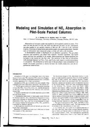
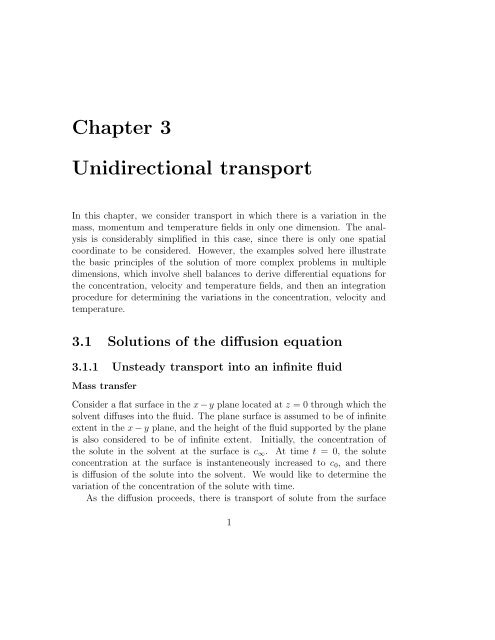
3.1. SOLUTIONS OF THE DIFFUSION EQUATION 3The conditions for T ∗ areMomentum transferT ∗ = 0as z → ∞ at all tT ∗ = 1 at z = 0 at all t > 0T ∗ = 0 at t = 0 for all z > 0 (3.6)The configuration consists of an infinite fluid in the z > 0 half space boundedby an infinite flat surface in the x − z plane. The fluid and the surface areinitially at rest. At time t = 0, the plane is instanteneously moved witha constant velocity U in the x direction. Determine the fluid velocity as afunction of time.As time proceeds, the momentum that is transported from the surfacediffuses through the fluid, resulting in fluid motion. However, the fluid ata large distance from the surface z → ∞ remains at rest. If u x is the fluidvelocity in the x direction, it is convenient to define a non-dimensional fluidvelocity u ∗ x = (u x /U). The conditions for the non-dimensional fluid velocityat the spatial boundaries of the flow and at initial time areShell balanceu ∗ x = 0u ∗ xas z → ∞ at all t= 1 at z = 0 at all t > 0u ∗ x = 0 at t = 0 for all z > 0 (3.7)In all three cases, the boundary and initial conditions 3.3, 3.6 and 3.7 areidentical in form. Since the transport in all three cases involves diffusion inthe direction perpendicular to the surface, and no variation along the surface,it is anticipated that the differential equation governing the transport willalso be identical in form. The differential equation for the concentration fieldis first derived using a shell balance, and the analogous equations for heatand momentum transfer are provided.Consider a shell of thickness ∆z in the z coordinate as shown in figure 3.1,and of thickness ∆x and ∆y in the x − y plane. There is a transport of massacross the surfaces of the shell due to diffusion, which results in a change inthe concentration in the shell. We consider the variation in the concentrationwithin this control volume over a time interval ∆t. Mass conservation

4 CHAPTER 3. UNIDIRECTIONAL TRANSPORTrequires that( ) () ()Accumulation of mass Input ofOutput of=−in the shellmass into shell mass from shell(3.8)The accumulation of mass in a time ∆t is given by( )Accumulation of mass= (c(x, y, z, t+∆t)−c(x, y, x, t))∆x∆y∆z (3.9)in the shellThe mass flux at the surface at z is given byj z = − D ∂c(3.10)∂z ∣ zand the mass entering the shell through the surface at z in a time interval∆t is given by the product of the mass flux, the area of transfer and the timeinterval ∆t,(Input ofmass into shell)= − ∆t∆x∆y(D ∂c∂z)∣ ∣∣∣∣z(3.11)In a similar manner, the mass leaving the surface at z + ∆z is given by()(Output of= − ∆t∆x∆y D ∂c )∣ ∣∣∣∣z+∆z(3.12)mass from shell∂zSubstituting equations 3.9, 3.11 and 3.12 into equation 3.8, and dividing by∆x∆y∆z∆t, we obtainc(x, y, z, t + ∆t) − c(x, y.z, t)= 1 (D ∂c− D ∂c)(3.13)∆t∆z ∂z ∣ z+∆z∂z ∣ zThe limit ∆t → 0 and ∆z → 0 is taken, to obtain a partial differentialequaiton for the concentration field.∂c∂t = ∂ (D ∂c )(3.14)∂z ∂zIf the diffusion coefficient is independent of the spatial position, the differentialequation 3.14 reduces to∂c∂t = D ∂2 c∂z 2 (3.15)

3.1. SOLUTIONS OF THE DIFFUSION EQUATION 5z−−>Infinityc*=0T*=0u*=0xz+ ∆ zzzz=0c*=1T*=1u*=1xxFigure 3.1: Configuration for similarity solution for unidirectional transport.The concentration equation 3.15 can also be expressed in terms of the scaledconcentration variable, c ∗ , defined in 3.2,∂c ∗∂t = D ∂2 c ∗∂z 2 (3.16)A similar shell balance procedure can be carried out for momentum transfer,and the equations for the temperature and velocity fields are∂T ∗∂t= ∂ (∂T ∗ )D T∂z ∂z(3.17)Though the final result for the momentum transfer process is exactlyanalogous to equations 3.16 and 3.17, the procedure is slightly different, andso we provide a brief outline of the calculation. First, note that there are

6 CHAPTER 3. UNIDIRECTIONAL TRANSPORTnow two directions in the problem. Since momemtum is a vector, there is adirection associated with the momentum itself, which is the x direction. Thesecond is the direction of diffusion, which is the z direction. The fundamentalbalance relation, equivalent of equation 3.8, is⎛⎜⎝Rate of change ofx momentumin the shell⎞⎟⎠ =(Sum of forcesin x direction)(3.18)The rate of change of momentum in the differential volume of thickness ∆zabout z in a time interval ∆t is given by,⎛⎜⎝Rate of change ofx momentumin the shell⎞⎟⎠ = ρ∆u x∆x∆y∆z∆t(3.19)The forces acting on the two surfaces at z and z +∆z are the products of theshear stress τ xz and the surface area (∆x∆y). It is important to keep trackof the directions of the forces in this case, since the force is a vector. Theshear stress τ xz is defined as the force per unit area in the x direction actingat a surface whose outward unit normal is in the positive z direction. For thesurface at z+∆z, the outward unit normal is in the +z direction, as shown infigure 3.1, and therefore the force per unit area at this surface is + τ xz | z+∆z.For the surface at z, the outward unit normal is in the −z direction, andtherefore the force per unit area at this surface is − τ xz | z. Finally, the rateof change of momentum, which is the change in momentum per unit time, isgiven by (ρ∆u x )(A∆z)/∆t. Therefore, the momentum balance equation is,(A∆z) ρ∆u x∆t= A(τ xz | z+∆z− τ xz | z) (3.20)Dividing throughout by A∆z, we obtain,ρ ∆u x∆t= τ xz| z+∆z− τ xz | z∆z(3.21)Taking the limit ∆t → 0 and ∆z → 0, we obtain the partial differentialequation,ρ ∂u x∂t= ∂τ xz∂z(3.22)

3.1. SOLUTIONS OF THE DIFFUSION EQUATION 7The shear stress is given by the product of the viscosity and the gradient ofthe velocity,∆u xτ xz = µ lim∆z→0 ∆z = µ∂u x(3.23)∂zWith this, the governing equation for the velocity field becomes,ρ ∂u x∂t= ∂ ∂z(µ ∂u x∂z)(3.24)Note that the differential equation derived above has the same form as theconcentration and energy diffusion equations 3.16 and 3.17, though it wasderived from a force balance. This indicates that the diffusion process is thesame for mass, momentum and energy. However, it should be noted thatmomentum could be transmitted by pressure forces in addition to viscousforces, and there is no analogue of pressure in mass and energy transport.When the velocity u x is scaled by U, the velocity of the bottom surface,the momentum equation becomes,∂u ∗ x∂t= ∂ ∂z(ν ∂u∗ x∂z)(3.25)where ν = (µ/rho) are the thermal and momentum diffusivities respectively.Solution procedureSince the conservation equations 3.16, 3.17 and 3.25 are identical in form, andthe boundary conditions 3.9, 3.11 and 3.12 are also identical, the same solutionprocedure can be used for all these, and the solutions for the concentration,velocity and temperature files, expressed in terms of the dimensionlessvariables c ∗ , T ∗ and u ∗ x, turn out to be identical.In order to solve the concentration equation 3.16 with the boundary condition3.9, it is first important to realise that there no intrinsic length scalein the problem, because the fluid and the flat plate are of infinite extent.Since the concentration c ∗ is dimensionless, there are only three dimensionalvariables z, t and D in the problem. These contain two dimensions, L and T ,and it is possible to construct only one dimensionless number, ξ = (z/ √ Dt).Therefore, just from dimensional analysis, it can be concluded that the concentrationfield does not vary independently with z and t, but only on thecombination ξ = (z/ √ Dt). If this inference is correct, it should be possible to

8 CHAPTER 3. UNIDIRECTIONAL TRANSPORTexpress the conservation equation 3.16 in terms of the variable ξ alone. Whenz and t are expressed in terms of ξ, the concentration equation becomes(−z2D 1/2 t 3/2 ) ∂c∗∂ξ = D Dt∂ 2 c ∗∂ξ 2 (3.26)After multiplying throughout by t, the equation for the concentration fieldreduces toξ ∂c ∗2 ∂ξ + ∂2 c ∗∂ξ = 0 (3.27)2Equation 3.27 validates the inference that the non-dimensionalised concentrationfield is only a function of ξ. It is also necessary to transform theboundary conditions 3.9 into conditions for the ξ coordinate. The transformedboundary conditions arec ∗ = 0 as z → ∞ at all t → as ξ → ∞c ∗ = 1 at z = 0 at all t > 0 → at ξ = 0c ∗ = 0 at t = 0 for all z > 0 → as ξ → ∞ (3.28)It is useful to note that the original conservation equation, 3.16, is a secondorder differential equation in z and a first order differential equation in t, andso this requires two boundary conditions in the z coordinate and one initialcondition. The conservation equation expressed in terms of ξ is a secondorder differential equation, which requires just two boundary conditions forξ. Equation 3.28 shows that one of the boundary conditions for z → ∞ andthe initial condition t = 0 turn out to be identical conditions for ξ → ∞,and therefore the transformation form (z, t) produces no inconsistency in theboundary and initial conditions.Equation 3.27 can be easily solved to obtain∫ ( )∞c ∗ (ξ) = C 1 + C 2 dξ ′ exp − ξ2ξ2(3.29)The constants C 1 and C 2 are determined from the conditions c ∗ = 1 at ξ = 0,and c ∗ = 0 for ξ → ∞, to obtainc ∗ (ξ) =√2π∫ ∞(z/ √ Dt)dξ ′ exp(− ξ22)(3.30)

3.1. SOLUTIONS OF THE DIFFUSION EQUATION 9From the solution 3.30, it can be inferred that there is no intrinsic lengthscale in the system, but the length scale for the z coordinate is a function oftime, and is proportional to √ Dt at time t. Thus, the length scale over whichdiffusion has taken place increases proportional to t 1/2 . Thus, equation 3.30will be a solution for the concentration diffusion in a configuration boundedby two plates, so long as the distance between the two plates L is largecompared to √ Dt.3.1.2 Steady diffusion into a falling filmThis problem is a simplification of the actual diffusion in a falling film, whichinvolves a combination of convection and diffusion. A thin film of fluid flowsdown a vertical surface. One side of the film is in contact with a gas whichis soluble in the liquid, and as the liquid flows down, the gas is dissolvedin the liquid. The concentration of gas in the liquid at the entrance is c ∞ ,while the concentration of gas at the liquid-gas interface is c 0 . The differencein concentration between the initial concentration in the liquid and theconcentration at the interface acts as a driving force for diffusion. The zcoordinate is perpendicular to the gas-liquid interface, which is located atz = 0. We also assume that the penetration depth for the gas into the liquid(to be determined a little later) is small compared to the thickness of theliquid film, so that the boundary conditions in the z coordinate given by 3.9are applicable. In addition, the boundary condition in the x coordinate isc = c ∞ at x = 0 (3.31)3.1.3 Diffusion in bounded channelsNext we consider the problem of diffusion in a channel bounded by two wallsseparated by a distance L, as shown in figure 3.2. Initially, the concentrationof the fluid in the channel is equal to c ∞ . At initial time, the concentrationof the solute on the wall at z = 0 is instanteneously increased to c 0 , whilethe concentration on the surface at z = L remains equal to c ∞ . The problemis to find the concentration field as a function of time. Similar problems canbe formulated for heat and momentum transfer.The concentration field is first expressed in terms of the scaled concentrationfield c ∗ by equation 3.2. The diffusion equation, obtained by a shellbalance as before, is given by equation 3.16. However, there is a modification

10 CHAPTER 3. UNIDIRECTIONAL TRANSPORTz+ ∆ zzz=Lc*=0T*=0u*=0xzz=0c*=1T*=1u*=1xxFigure 3.2: Configuration for similarity solution for unidirectional transport.in the boundary conditions,c ∗ = 0at z = L at all tc ∗ = 1 at z = 0 at all t > 0c ∗ = 0 at t = 0 for all z > 0 (3.32)In this case, it is not possible to effect a reduction to a similarity form,because there is an additional length scale L in the problem, and so the zcoordinate can be scaled by L. A scaled z coordinate is defined as z ∗ = (z/L),and the diffusion equation in terms of this coordinate is∂c ∗∂t = D L 2 ∂ 2 c ∗∂z ∗2 (3.33)The above equation suggests that it is appropriate to define a scaled timecoordinate t ∗ = (Dt/L 2 ), and the conservation equation in terms of thisscaled time coordinate is∂c ∗∂t = ∂2 c ∗(3.34)∗ ∂z ∗2The boundary conditions, in terms of the scaled coordinates z ∗ and t ∗ , arec ∗ = 0at z ∗ = 1 at all t ∗

3.1. SOLUTIONS OF THE DIFFUSION EQUATION 11c ∗ = 1 at z ∗ = 0 at all t ∗ > 0c ∗ = 0 at t ∗ = 0 for all z ∗ > 0 (3.35)It is expected that in the long time limit, t ∗ → ∞, the concentration fieldwill attain a steady state value c ∗ s which is independent of time. This steadystate concentration field is obtained by solving 3.16 with the time derivativeset equal to zero, and the solution for the steady concentration field is alinear concentration profile,c ∗ = C 1 z ∗ + C 2 (3.36)The constants C 1 and C 2 are obtained from the boundary conditions at z ∗ = 0and z ∗ = 1,c ∗ s = (1 − z∗ ) (3.37)The variation of concentration with time can be determined by dividingthe concentration into a steady and an unsteady part,c ∗ = c ∗ s + c∗ u , (3.38)where c ∗ u is the difference between the actual concentration and the concentrationat steady state. The reason for this decomposition will become cleara little later. The conservation equation for the unsteady concentration fieldis identical to that for the original concentration field, because (∂c ∗ s /∂t∗ ) = 0and (∂ 2 c ∗ s /∂z∗2 ) = 0,∂c ∗ u∂t = ∂2 c ∗ u(3.39)∗ ∂z ∗2However, the boundary condition for c ∗ u is different from that for the c∗ , andis obtained by subtracting c ∗ s from c∗ at the boundaries,c ∗ u = 0at z ∗ = 1 at all t ∗c ∗ u = 0 at z∗ = 0 at all t ∗ > 0c ∗ u = −c∗ s at t ∗ = 0 for all z ∗ > 0 (3.40)Equation 3.16 can be solved by the method of ‘separation of variables’,where the unsteady concentration field is expressed as two functions, one ofwhich is only a function of t ∗ , while the other is only a function of z ∗ .c ∗ u = Θ(t∗ )Z(z ∗ ) (3.41)

12 CHAPTER 3. UNIDIRECTIONAL TRANSPORTThis is inserted into the conservation equation 3.16, and the equation isdivided by the production ΘZ, to obtain1 dΘΘ dt = 1 d 2 Z(3.42)∗ Z dz ∗2In equation 3.42, the left side is only a function of t ∗ , while the right sideis only a function of z ∗ . From this, it can be inferred, as follows, that thesetwo functions have to be constants independent of z ∗ and t ∗ . To infer this,assume that these two functions are not constants, and that the left sidevaries as t ∗ is varied, and the right side varies as z ∗ is varied. In this case,if we keep z ∗ a constant and vary t ∗ , then the left side of 3.42 varies, whilethe right side remains a constant, and so the equality is destroyed. The onlyway for the equality to hold, if the left side is only a function of t ∗ and theright side is only a function of z ∗ , is if the two sides are constants.The solution for Z is first obtained by solving1 d 2 ZZ dz = ∗2 −α2 (3.43)where α is a positive constant. The reason for choosing the right side of3.43 to be negative will become apparent a little later. The solution for thisequation isZ = C 1 sin (αz ∗ ) + C 2 cos (αz ∗ ) (3.44)where C 1 and C 2 are constants to be determined from the boundary conditions.The boundary condition c ∗ u = 0 (Z = 0) at z ∗ = 0 is satisfied forC 2 = 0. The boundary condition ca u = 0 at z ∗ = 1 is satisfied if α = (nπ).Therefore, the solution for Z which satisfied the boundary conditions in thez ∗ coordinate isZ = C 1 sin (nπz ∗ ) (3.45)where n is an integer.The solution for Θ can now be obtained from the equationThis equation is solved to obtain1 dΘΘ dt = ∗ −α2 = −n 2 π 2 (3.46)Θ = C 3 exp (−n 2 π 2 t ∗ ) (3.47)

14 CHAPTER 3. UNIDIRECTIONAL TRANSPORT3.1.4 Unsteady diffusion in a cylinderA cylindrical container of radius R containing fluid with temperature T ∞ isdipped into a bath of fluid containing solute with temperature T 0 . Assumethat the bath is large enough that the conduction of heat into the fluid doesnot appreciably change the temperature of the bath, and that there is noresistance to heat transfer in the walls of the container. The temperature inthe cylinder as a function of time and position is to be determined.A cylindrical coordinate system is used, as shown in figure 3.3, where zis the axial coordinate and r is the radial coordinate. There is no variationof temperature in the z coordinate, since the cylinder is considered to be ofinfinite extent. In order to obtain a differential equation for the temperaturevariation in the cylinder, a shell of thickness ∆r and height ∆z at radius ris considered. The terms in the balance equation 3.8 for the energy in thecylindrical shell are as follows.( )Accumulation of energy= ρCin the shellp (T (x, y, z, t+∆t)−T (x, y, x, t))2πr∆r∆z(3.53)The total energy entering the shell at r is the product of the heat flux, thesurface area, and the time interval ∆t,(Input ofenergy into shell) (= − K ∂T )(2πr∆z∆t)(3.54)∂r∣ rSimilarly, the total energy leaving the shell at r + ∆r is() (Output of= − K ∂T )(2πr∆z∆t)(3.55)energy from shell∂r∣ r+∆rWhen these are inserted into the conservation equation 3.8, and divided by∆r∆t, the net energy balance for the shell is(T (x, y, z, t + ∆t) − T (x, y, x, t))ρC p r = 1 (Kr ∂T− Kr ∂T)∆t∆r ∂r ∣ r+∆r∂r ∣ r(3.56)Taking the limit ∆r → 0 and ∆t → 0, the partial differential equation forthe temperature field is∂T∂t = D (T ∂r ∂T )(3.57)r ∂r ∂r

3.1. SOLUTIONS OF THE DIFFUSION EQUATION 15R∆ rrT*=0∆ zzrFigure 3.3: Heat diffusion into a cylinder.It is important to note that there is a variation in the surface area of theshell as r varies, and there is a variation in the total energy transportedthrough the shell due to the variation in this surface area. This leads to amore complicated form for the diffusion term in 3.57, in comparison to thesecond derivative encountered in the diffusion from a flat plane, 3.17.The conservation equation 3.57 can be scaled as follows. The scaledtemperature field is defined by equation 3.5, while the scaled distance andtime coordinates are defined as r ∗ = (r/R) and t ∗ = (tR 2 /D T ), since Ris the length scale in the radial direction. The conservation equation 3.57,expressed in these coordinates, is∂T ∗∂t = 1 (∂r ∗ ∂T ∗ )∗ r ∗ ∂r ∗ ∂r ∗(3.58)

16 CHAPTER 3. UNIDIRECTIONAL TRANSPORTThe boundary conditions areT ∗ = 0at r ∗ = 1 for all t ∗T ∗ = 1 at t ∗ = 0 for all r ∗∂T ∗∂r = 0 ∗ at r∗ = 0 for all t ∗ (3.59)Equation 3.58 is solved using the method of separation of variables. Thefinal steady state solution is one in which the temperature is uniform, T ∗ = 0,throughout the cylinder. The unsteady solution is solved using the substitutionT ∗ = R(r ∗ )Θ(t ∗ ) (3.60)where R is a function of the radial coordinate, and Θ is a function of time.The form 3.60 is inserted into the temperature equation, 3.58, and the resultingequation is divided by R(r ∗ )Θ(t ∗ ) to obtain1 ∂ΘΘ ∂t = 1 ∗ R1r ∗(∂r ∗ ∂R )∂r ∗ ∂r ∗(3.61)The left side of the above equation is only a function of time, while the rightside is only a function of r ∗ . Therefore, the equality can only be satisfied ifboth sides are equal to constants. The right side of the above equation isfirst solved,(1 d 2 RR dr + 1 )dR= −α 2 (3.62)∗2 r ∗ dr ∗A special function solution for equation 3.62 can be obtained by recastingthe equation asr ∗2 d2 R dR+ r∗dr∗2 dr + ∗ α2 r ∗ R = 0 (3.63)The solution of the above equation is in the form of ‘Bessel functions’,R = C 1 J 0 (αr ∗ ) + C 2 Y 0 (αr ∗ ) (3.64)The values of the constants C 1 and C 2 are determined from the boundaryconditions at r ∗ = 0 and r ∗ = 1. At r ∗ = 0, the radial derivative of J 0 (αr ∗ ) isidentically zero, whereas the radial derivative of Y 0 (αr ∗ ) approaches infinityfor r ∗ → 0. Therefore the boundary condition at r ∗ = 0 can be satisfied only

3.1. SOLUTIONS OF THE DIFFUSION EQUATION 17if C 2 = 0. The second boundary condition, T ∗ = 0 at r ∗ = 1, is used todetermine the value of α in equation 3.62,J 0 (α) = 0 (3.65)There are multiple solutions for this equation, the first few of which are givenby. The equation for Θ,1 dΘΘ dt = ∗ −α2 n (3.66)can be solved to obtainΘ = exp (−αn 2 t∗ ) (3.67)With this, the solution for the temperature field is∞∑T ∗ = C n J 0 (α n r ∗ ) exp (−αn 2 t∗ ) (3.68)n=1The coefficients C n should satisfy the initial condition at t ∗ = 0,∞∑C n J 0 (α n r ∗ ) = 1 (3.69)n=1The values of the coefficients can be determined using orthogonality conditionsfor the Bessel functions, which in this case are∫ 10r ∗ dr ∗ J 0 (α n r ∗ )J 0 (α m r ∗ ) = 1 2 (J 1(α n )) 2 for m = n= 0 for m ≠ n (3.70)In order to determine the coefficients, the right and left sides of 3.70 aremultiplied by r ∗ J 0 (α m r ∗ ), and integrated from r ∗ = 0 to r ∗ = 1, to obtain3.1.5 Oscillatory flow∫112 (J 1(α n )) 2 C n = r ∗ dr ∗ J 0 (α n r ∗ ) (3.71)0This example is used to illustrate the use of complex variables in problemswhere the forcing on the fluid is oscillatory in time. Consider the flat platebounding a fluid in the half space z > 0, shown in figure 3.4, with the

18 CHAPTER 3. UNIDIRECTIONAL TRANSPORTmodification that the plate has an oscillatory velocity U = U 0 cos (ωt). Thedifferential equation for the velocity field is given by equation 3.25,∂u x∂t= ν ∂2 u x∂z 2 (3.72)The boundary conditions in this case, analogous to 3.7, areu x = U cos (ωt) at z = 0u x = 0 at z = L (3.73)The solution procedure is simplified if the boundary condition is recast asfollows. The ‘complex’ velocity field u † x is defined as a velocity field thatsatisfies the same differential equation as 3.72,∂u † x∂tbut which satisfies the boundary conditions= ν ∂2 u † x∂z 2 (3.74)u † x = U exp (ıωt) at z = 0u † x= 0 at z = L (3.75)where ı is the square root of −1. It is apparent that the solution to thedifferential equation 3.74, with the boundary condition 3.75, is the real partof the solution to the differential equation 3.72 with the boundary condition3.73. Since dealing with exponential functions is easier than dealing withsines and cosines, it is more convenient to solve equation 3.74 with boundaryconditions 3.75 for u † x , and then take the real part of the solution to obtainthe solution u x of equation 3.72.The non-dimensional velocity u †∗x is defined as u†∗ x = (u† x /U), while thescaled z and time coordinates are defined as z ∗ = (z/L) and t ∗ = (tν/L 2 ).The momentum conservation equation and boundary conditions in terms ofthis scaled velocity are∂u †∗x∂t = ∂2 u †∗x(3.76)∗ ∂z ∗2u †∗x = exp (ω∗ t ∗ ) at z = 0= 0 at z = L (3.77)u †∗x

3.1. SOLUTIONS OF THE DIFFUSION EQUATION 19z−−>Infinityu*=0~xz+ ∆ zzzz=0u*=1~xux=U cos( ω t)Figure 3.4: Oscillatory flow at a flat surface.xwhere the scaled frequency is given by ω ∗ = (ωL 2 /ν).The differential equation 3.76 for the velocity field is a linear differentialequation, since all terms in the equation contain only the first power of u †∗x .This first order differential equation is driven by a wall which is oscillatorywall velocity with scaled frequency ω ∗ . When a linear system is driven bywall motion of frequency ω ∗ , the response of the system also has the samefrequency ω ∗ . (This is not true if the system is non-linear, since forcing of acertain frequency will generate response at different harmonics of this basefrequency). Therefore, the time dependence of the velocity field in the fluidcan be considered to be of the formu †∗x = ũ∗ x (z∗ ) exp (ıω ∗ t ∗ ) (3.78)When this form is inserted into the differential equation 3.76, and divided byexp (ıω ∗ t ∗ ), the resulting equation is an ordinary differential equation for ũ ∗ x .The boundary conditions for ũ ∗ x (3.77) becomeıω ∗ ũ ∗ x = ∂2 ũ ∗ x∂z ∗2 (3.79)ũ ∗ x = 1 at z = 0

20 CHAPTER 3. UNIDIRECTIONAL TRANSPORTũ ∗ xThis equation is easily solved to obtain= 0 at z = L (3.80)ũ ∗ x (z∗ ) = C 1 exp ( √ ıω ∗ z ∗ ) + C 2 exp (− √ ıω ∗ z ∗ ) (3.81)where C 1 and C 2 are determined from the boundary conditions at z ∗ = 0and z ∗ = 1,ũ ∗ x (z∗ ) = exp (√ ıω ∗ z ∗ ) − exp ( √ ıω ∗ (2 − z ∗ ))1 − exp (2 √ ıω ∗ )(3.82)The physical velocity field, which is the real part of the product of ũ ∗ x andexp (ıω ∗ t ∗ ), is[ √exp (u ∗ x(z ∗ ıω∗ z ∗ ) − exp ( √ ıω) = Real∗ (2 − z ∗ ]))1 − exp (2 √ exp (ıω ∗ t ∗ ) (3.83)ıω ∗ )Before solving the above equation, it is useful to examine some limitingcases for the frequency of oscillation. In the limit ω ∗ → 0, the solution forthe fluid velocity, 3.83, isu ∗ x(z ∗ ) = (1 − z ∗ ) exp (ıω ∗ t ∗ ) (3.84)The physical reason for this result is as follows. The scaled frequency ofoscillation is obtained by dividing the frequency, ω, by the inverst of thetime required for the momentum to diffuse across the length of the channel,(L 2 /ν). If the scaled frequency ω ∗ is small, then the time period of variationof the velocity of the bottom plate is long compared to the time required formomentum to diffuse across the channel. In this case, it is expected, thatthe velocity profile at any time instant along the oscillation cycle is identicalto the velocity for a flow driven by a steady plate velocity which is equal tothe instanteneous value of the plate velocity at that instant in the cycle. Inthe limit ω ∗ ≫ 1, the fluid velocity field is given byu ∗ x(z ∗ ) = exp (− √ ıω ∗ z ∗ ) (3.85)In this case, the velocity field decreases over a distance z ∗ ∼ (1/ √ ω ∗ ) fromthe surface. This is because the frequency of oscillation is large comparedto the time required for diffusion of momentum across the channel, and themomentum diffuses only to a distance comparable to (L/ √ ω ∗ ). Beyond thisdistance, the momentum generated during the positive and negative parts ofa cycle cancel out, and the fluid velocity approaches zero.

3.2. EFFECT OF BULK FLOW AND REACTION IN MASS TRANSFER21z=LDry airzz=0¡¡¡¢¡¢¡¢¡¢¢¡¢¡¢¡¢¡ ¡ ¡Water¡¡¡¢¡¢¡¢¡¢¢¡¢¡¢¡¢¡ ¡ ¡¡¡¡¢¡¢¡¢¡¢¡ ¡ ¡x¢¡¢¡¢¡¢¡ ¡ ¡¢¡¢¡¢¡¢Figure 3.5: Diffusion with bulk flow.3.2 Effect of bulk flow and reaction in masstransferIn this section, the special effects of bulk flow and reactions on the solutionsfor unidirection mass transfer problems are examined.3.2.1 Diffusion in a stagnant filmWater evaporates from a container through a stagnant air film through aglass tube into dry air flowing at the top of the tube, as shown in figure 3.5.If the mole fraction at the surface of the liquid surface is the saturation molefraction x W s , and the dry air flowing past the tube does not contain anywater, what is the concentration profile of water in the glass tube?Though the air in the tube is stationary, the mean velocity across anyhorizontal surface in the tube is not zero, because of the flow of water vapour

22 CHAPTER 3. UNIDIRECTIONAL TRANSPORTacross the surface. The flux of water across a surface, j W z , contains a componentdue to the bulk flow, as well as a component due to the diffusion ofwater across the surface.j W z = −cD W Adx Wdz + x W (j W z + j Az ) (3.86)The last term on the right side of equation 3.86 is the flux of water due to thebulk flow, where the total molar flow rate is the sum of the fluxes of water(j W z ) and air (j Az ). In this particular case, the flux of air is identically zero,and so the flux of water vapour across a surface is given byj W z = −c dx W1 − x W dz(3.87)The mass balance equation is obtained by writing a flux balance across asection of thickness ∆z of the tube, which at steady state provides,j W z | z+∆z− j W z | z= 0 (3.88)If the above equation is divided by ∆z the differential equation for the fluxin the limit ∆z → 0 isdj W z= d ()1 dx W= 0 (3.89)dz dz 1 − x W dzThis equation is solved to obtain− log (1 − x W ) = A 1 z + A 2 (3.90)The constants A 1 and A 2 are determined from the boundary conditions x W =x W s at z = 0 and x = 0 at z = l,( ) z/l(1 − x W ) (1 −(1 − x W s ) = xW f )(3.91)(1 − x W s )3.2.2 Diffusion with homogeneous reactionA gaseous reactant A dissolves in a liquid B, and undergoes a first orderreaction A+B → AB, in a tank of height L, as shown in figure 3.6. The massbalance equation, 3.14 has to be modified in this case due to the presence of

3.3. EFFECT OF PRESSURE ON MOMENTUM TRANSPORT 23a ‘consumption’ term due to chemical reaction. The mass balance equationat steady state takes the formj Az | z− j Az | z+∆z− kc A S∆z = 0 (3.92)This can be reduced to a differential equation by dividing throughout byS∆z, and taking the limit ∆z → 0,dj Azdz − kC A = 0 (3.93)If the concentration of A is small, the flux of A is given byj Az = −D ABdc AdzInserting this into the concentration equation 3.93, we get(3.94)The boundary conditions are−D ABd 2 c Adz 2 + kC A = 0 (3.95)c A = c A0 at z = 0The solution that satisfied both these conditions isj Az = 0 at z = L (3.96)C AC A0= cosh ((kL2 /D AB ) 1/2 (1 − (z/L)))cosh (kL 2 /D AB ) 1/2 (3.97)3.3 Effect of pressure on momentum transportThe momentum balance condition states that the rate of change of momentumis equal to the applied force.[] [] []Rate ofRate ofSum of forces−+= 0momentum in momentum out acting on the system(3.98)

24 CHAPTER 3. UNIDIRECTIONAL TRANSPORTc=c at z=0z=0z+ ∆ zzz=Lj =0 at z=LzFigure 3.6: Diffison with homogeneous chemical reaction.

3.3. EFFECT OF PRESSURE ON MOMENTUM TRANSPORT 25This balance equation is written for a control volume of fluid which is in theform of a thin shell. Momentum enters or leaves the control volume due tofluid flow into or out of the control volume, or due to the stresses acting onthe surface due to viscosity. The forces acting on the system are usually thegravitational force or the centrifugal force. Momentum balances are usuallyeasy to apply only if the streamlines are straight. Applying momentumbalances to systems with curved streamlines is more difficult, as we shall seein the last example of this section.The procedure for solving problems with momentum balance is to writethe momentum balance equation for a shell of finite thickness, and thenlet the thickness go to zero. In this limit, the difference equations for thevelocity field across a finite shell reduces to differential equations for thevelocity fields. These can then be solved, subject to appropriate boundaryconditions, in order to determine the velocity fields.The boundary conditions generally involve specifying the velocity or stressfields at the boundaries of the flow. These conditions depend on the surfaceadjoining the liquid at its boundaries.1. If there is a solid surface adjacent to the fluid, the appropriate boundarycondition is the ‘no slip’ condition which states that the velocity of thefluid at the surface is equal to the velocity of the surface itself.2. At a liquid - gas interface, the momentum flux, and consequently thevelocity gradient, in the liquid side is assumed to be zero, because theviscosity of the gas is small compared to that of the liquid.3. At a liquid - liquid interface, the momentum flux and the velocity arecontinuous across the interface.Falling filmWe first consider the flow of a falling film along an inclined plane, as shownin figure 3.7. This type of flow is often encountered in cooling towers, evaporationchambers and gas absorption equipment. The plane is inclined atan angle β to the vertical, and we consider a section L of the film which issufficiently far removed from the entrance and exit that the velocity profileis independent of variation in the z direction along the flow. The only non -zero component of the velocity, u z , is a function of the coordinate x alone.

26 CHAPTER 3. UNIDIRECTIONAL TRANSPORTz=0z=Lv (x)z¡¡¡¡¡¡¡¡¡¡¡¡¡¡¡¡¡¡¡¡¡¢¡¢¡¢¡¢¡¢¡¢¡¢¡¢¡¢¡¢¡¢¡¢¡¢¡¢¡¢¡¢¡¢¡¢¡¢¡¢¡¢¡¢¡¢gzz+ ∆ z¡¡¡¡¡¡¡¡¡¡¡¡¡¡¡¡¡¡¡¡¡¢¡¢¡¢¡¢¡¢¡¢¡¢¡¢¡¢¡¢¡¢¡¢¡¢¡¢¡¢¡¢¡¢¡¢¡¢¡¢¡¢¡¢¡¢¡¡¡¡¡¡¡¡¡¡¡¡¡¡¡¡¡¡¡¡¡¢¡¢¡¢¡¢¡¢¡¢¡¢¡¢¡¢¡¢¡¢¡¢¡¢¡¢¡¢¡¢¡¢¡¢¡¢¡¢¡¢¡¢¡¢¢¡¢¡¢¡¢¡¢¡¢¡¢¡¢¡¢¡¢¡¢¡¢¡¢¡¢¡¢¡¢¡¢¡¢¡¢¡¢¡¢¡¢¡¢ ¡ ¡ ¡ ¡ ¡ ¡ ¡ ¡ ¡ ¡ ¡ ¡ ¡ ¡ ¡ ¡ ¡ ¡ ¡ ¡ ¡ ¡¡¡¡¡¡¡¡¡¡¡¡¡¡¡¡¡¡¡¡¡¢¡¢¡¢¡¢¡¢¡¢¡¢¡¢¡¢¡¢¡¢¡¢¡¢¡¢¡¢¡¢¡¢¡¢¡¢¡¢¡¢¡¢¡¢¡¡¡¡¡¡¡¡¡¡¡¡¡¡¡¡¡¡¡¡¡¢¡¢¡¢¡¢¡¢¡¢¡¢¡¢¡¢¡¢¡¢¡¢¡¢¡¢¡¢¡¢¡¢¡¢¡¢¡¢¡¢¡¢¡¢¡¡¡¡¡¡¡¡¡¡¡¡¡¡¡¡¡¡¡¡¡¢¡¢¡¢¡¢¡¢¡¢¡¢¡¢¡¢¡¢¡¢¡¢¡¢¡¢¡¢¡¢¡¢¡¢¡¢¡¢¡¢¡¢¡¢¡¡¡¡¡¡¡¡¡¡¡¡¡¡¡¡¡¡¡¡¡¢¡¢¡¢¡¢¡¢¡¢¡¢¡¢¡¢¡¢¡¢¡¢¡¢¡¢¡¢¡¢¡¢¡¢¡¢¡¢¡¢¡¢¡¢¡¡¡¡¡¡¡¡¡¡¡¡¡¡¡¡¡¡¡¡¡¢¡¢¡¢¡¢¡¢¡¢¡¢¡¢¡¢¡¢¡¢¡¢¡¢¡¢¡¢¡¢¡¢¡¢¡¢¡¢¡¢¡¢¡¢¢¡¢¡¢¡¢¡¢¡¢¡¢¡¢¡¢¡¢¡¢¡¢¡¢¡¢¡¢¡¢¡¢¡¢¡¢¡¢¡¢¡¢¡¢¡ ¡ ¡ ¡ ¡ ¡ ¡ ¡ ¡ ¡ ¡ ¡ ¡ ¡ ¡ ¡ ¡ ¡ ¡ ¡ ¡¢¡¢¡¢¡¢¡¢¡¢¡¢¡¢¡¢¡¢¡¢¡¢¡¢¡¢¡¢¡¢¡¢¡¢¡¢¡¢¡¢¡¢¡¢ ¡ ¡ ¡ ¡ ¡ ¡ ¡ ¡ ¡ ¡ ¡ ¡ ¡ ¡ ¡ ¡ ¡ ¡ ¡ ¡ ¡ zx¡¡¡¡¡¡¡¡¡¡¡¡¡¡¡¡¡¡¡¡¡¢¡¢¡¢¡¢¡¢¡¢¡¢¡¢¡¢¡¢¡¢¡¢¡¢¡¢¡¢¡¢¡¢¡¢¡¢¡¢¡¢¡¢¡¢Figure 3.7: Flow down an inclined plane.

3.3. EFFECT OF PRESSURE ON MOMENTUM TRANSPORT 27A momentum balance is set up for a thin shell of fluid of thickness ∆xbounded by the planes z = 0 and z = L. The various components of themomentum balance in the z direction areRate of zmomentum inacross surfaceat xRate of zmomentum outacross surfaceat x + ∆xRate of zmomentum inacross surfaceat z = 0Rate of zmomentum outacross surfaceat z = LGravity forceacting onthe fluid(LW ) −τ xz | x(LW ) −τ xz | x+∆x(W ∆xv z ) ρv z | z=0(W ∆xv z ) ρv z | z=L(W L∆x)(ρg cos (β) (3.99)When these terms are substituted into the momentum balance equation, weget−LW τ xz | x+LW τ xz | x+∆x+W ∆ x ρvz2 ∣ −W ∆ x ρv 2 z=0z∣ +LW δxW g cos (β) = 0z=L(3.100)Dividing throughout by LW ∆x and taking the limit as ∆x → 0, we get( )τxz |lim x+∆x− τ xz | x+ ρg cos (β) = 0 (3.101)∆x→0 ∆xThe first term on the left of the above equation is the derivative of the shearstress, and so this can be written asdτ xzdx+ ρg cos (β) = 0 (3.102)

28 CHAPTER 3. UNIDIRECTIONAL TRANSPORTThis can be integrated to giveτ xz = −ρg cos (β)x + C 1 (3.103)where C 1 is a constant of integration. The constant of integration can be determinedby making use of the boundary condition at the liquid gas interfaceWith this, the equation for the shear stress becomesτ xz = 0 at x = 0 (3.104)τ xz = −ρg cos (β)x (3.105)If the fluid is Newtonian, the momentum flux is related to the velocitygradient byτ xz = µ dv z(3.106)dxThis is easily integrated to give an expression for the velocity( ) ρg cos (β)v z = −x 2 + C 2 (3.107)2µThe constant of integration can be determined using the condition that atx = h, v z = 0, since the surface at x = h is a solid surface and a noslip boundary condition is applicable here. With this, the equation for thevelocity profile is[ ( ]v z = ρgh2 cos (β) x 21 −(3.108)2µh)Hence the velocity profile is a parabolic profile.Various parameters can be determined once this velocity profile is known.1. the maximum velocity, v zm , is clearly at x = 0v zm = ρgh2 cos (β)2µ(3.109)2. The total flow rate is determined fromQ =∫ h0dx∫ W0dyv z= ρgW h3 cos (β)3µ(3.110)

3.3. EFFECT OF PRESSURE ON MOMENTUM TRANSPORT 293. The mean velocity can be calculated from〈v z 〉 = Q h= ρgW h2 cos (β)3µ(3.111)4. The film thickness δ can be expressed in terms of the flow rate as() 1/33µQh =(3.112)ρgW cos (β)5. The total force on the inclined surface in the z direction is given byF =∫ L0dz∫ W0dy τ xz | x=h(3.113)= ρghLW cos (β) (3.114)This is just equal to the weight of the fluid in the z direction understeady flow conditions.The momentum balance equation in the x direction can also be writtenin an analogous fashion.Rate of xmomentum inacross surfaceat xRate of xmomentum outacross surfaceat x + ∆xGravity forceacting onthe fluid(LW ) −τ xx | x(LW ) −τ xx | x+∆x(W L∆x)(ρg sin (β) (3.115)The momentum balance equation obtained from the above equation is−LW τ xx | x+ LW τ xx | x+∆x+ LW δxW g sin (β) = 0 (3.116)

30 CHAPTER 3. UNIDIRECTIONAL TRANSPORT∆ xR∆ rrrxFigure 3.8: Flow in a circular tube.Since τ xx = −p for a Newtonian fluid, the above equation reduces todpdx= ρg sin (β) (3.117)The variation in the pressure in the film is then given byp = ρgx sin (β) (3.118)The above analytical results are valid only if the flow is laminar andthe streamlines are smooth, so that the flow can be considered steady. Theseconditions are satisfied for the slow viscous flow of a thin film. As the velocityincreases or the film thickness increases, it has been found that there is atransition from a laminar flow ith straight streamlines to a laminar flow withrippling and then to a turbulent flow. The conditions under which thesetransitions occur is determined by the ‘Reynolds number’, Re = 4h〈v z 〉ρ/µ.A laminar flow without rippling is observed for Re < 10, while there isrippling for 10 < Re < 1000. The flow becomes turbulent when the Reynoldsnumber increases beyond about 1000.Example: Flow through a circular tube.The flow through a circular tube is often encountered in engineering applications,and the laminar flow can be analysed using shell momentum balances.The only new feature here is the cylindrical coordinate system that isused for the analysis, as shown in figure 3.8.Consider a cylindrical shell of thickness ∆r and length ∆x. The balance

3.3. EFFECT OF PRESSURE ON MOMENTUM TRANSPORT 31equation for the x component of the momentum can be written as,Rate of changeof x momentum= Sum of forces l (3.119)The rate of change of momentum in a time interval ∆t within the differentialvolume under consideration can be written as,Rate of changeof x momentum = ∆(ρu x)(2πr∆r∆z (3.120)∆twhere ∆(ρu x ) is the change in the momentum per unit volume in the timeinterval ∆t.There are four bounding surfaces for the differential volume under consideration,two or which are at perpendicular to the x axis and located atx and x + ∆x, and two of which are perpendicular to the radial co-ordinateand are located at r and r + ∆r. The forces acting on the surfaces at x andx + ∆x can be separated into two parts, the first due to the pressure actingon the surfaces, and the second due to the flux of momentum due to fluidmotion. The forces due to fluid pressure can be written as,Force due to pressureon surface at xForce due to pressureon surface at x + ∆x= p(r, θ, x)(2πr∆r)= −p(r, θ, x + ∆x)(2πr∆r) (3.121)Note that there is a negative sign for the force at x+∆x, because the pressurealways acts along the inward unit normal at the surface, and the inward unitnormal at x + ∆x is in the negative x direction. There is an additional forcedue to the flow of momentum into the differential volume through the surfaceat x and the flow of momentum out of the differential volume through thesurface at x + ∆x. This force is given by the product of the momentum flux(momentum transported per unit area per unit time) and the surface area.The momentum flux is the product of the momentum density (ρu x ) (per unitvolume) and the normal velocity to the surface u x . This is analogous to themass flux, which is the product of the concentration (mass density) c andthe normal velocity. Therefore, the force due to the flow of momentum is,Force due to momentum flowon surface at xForce due to momentum flowon surface at x + ∆x= ((ρu x )u x (2πr∆r)= −p(r, θ, x + ∆x)(2πr∆r)(3.122)

32 CHAPTER 3. UNIDIRECTIONAL TRANSPORTNote that the force at (x + ∆x) is negative, since momentum leaves thedifferential volume at this surface. We can now add up all the contributionsto get−2πrLτ rz | r+2πrLτ rz | r+∆r+2πr∆rρvz2 ∣ −2πr∆rρv 2 ∣z=0z∣ z=L+2πr∆rLρg+2πr∆r(p 0 −p L ) = 0(3.123)Since the fluid is considered to be incompressible, v z is equal at z = 0 andz = L. Therefore, the momentum flux due to fluid motion cancels out, andwe can divide by 2πL∆r and take the limit ∆r → 0 to get1 d(rτ rz )+r dr( ) P0 − P L= 0 (3.124)Lwhere P = p − ρgz. This equation can be integrated once to giveτ rz = −( ) P0 − P Lr + C 12L r(3.125)If the momentum flux is not infinite at r = 0, the constant C 1 is zero and sowe get( ) P0 − P Lτ rz = −r (3.126)2LThe velocity profile is calculated from the relationThis is used to obtainv z = −τ rz = µ dv zdr(3.127)( ) P0 − P Lr 2 + C 2 (3.128)4LThe constant C 2 is determined from the condition that the fluid velocity iszero at the wall, v z = 0 at r = R.v z =( (P0 − P L )R 2 ) ( )1 − r24µLR 2(3.129)This is the familiar parabolic velocity profile for the flow in a tube. Thevelocity is a maximum at the center, and decreases to zero at the walls. Theshear stress ia a maximum at the walls and decreases to zero at the center.

3.3. EFFECT OF PRESSURE ON MOMENTUM TRANSPORT 33The volumetric flow rate is determined by integrating the velocity profileover the radius of the tube.Q = π(P 0 − P L )R 48µL(3.130)This shell balance analysis is also valid only for steady flows, where thestreamlines are straight. This occurs in a fully developed flow, away fromthe entrance or exit of the pipe, and also in a the Reynolds number is lessthan 2100, where the Reynolds number is defined as Re = ρv max R/µ, wherev max is the maximum velocity and R is the radius of the pipe.Oscillatory flow in a pipeAn oscillatory pressure gradient (∆p/L) = k cos (ωt) is applied across a pipeof length L. Determine the velocity profile in the pipe.The differential equation for the velocity profile is, The momentum equationin the flow x direction is∂u x∂t − 1 Re( ∂ 2 u x∂x 2)+∂2 u x= − ∂p∂r 2 ∂x(3.131)Setting u r = 0 for a unidirectional flow, and neglecting variations in thestreamwise direction, the equation for the velocity profile is∂u x∂t − 1 ( 1 dRe r dr r du )x= − cos (t) (3.132)drwhere Re = (ρωR 2 /µ). Use the solution for an oscillatory flow,The equation for ũ x becomesıũ x − 1 Reu x = ũ x exp (ıt) (3.133)( 1rddr r dũ )x= 1 (3.134)drThe solution for ũ x is divided into a homogeneous and a particular solution.The homogeneous solution is given byũ xh = CJ 0 ( √ −ıRer) (3.135)

34 CHAPTER 3. UNIDIRECTIONAL TRANSPORTzxFigure 3.9: Flow of immiscible fluids.where J 0 is the Bessel function. The particular solution is given byũ xp = −ı (3.136)The complete solution is⎛ũ x = ı ⎝ J 0( √ ⎞−ıωr)√J 0 ( −ıω) − 1 ⎠ (3.137)Adjacent flow of two immiscible liquids.This is an example which illustrates the application of boundary conditionsbetween two immiscible liquids. Two immiscible liquids flow through a channelof length L and width W under the influence of a pressure gradient, asshown in figure 3.9. The flow rates are adjusted such that the channel is halffilled with fluid I (more dense phase) and half filled with fluid II (less densephase). It is necessary to find the distribution or velocity in this case.The momentum balance is similar to that for the flow in a pressure gradientshown in the last example. The pressure balance reduces todτ xzdx + p 0 − p L= 0 (3.138)LThis equation is valid in either phase I or phase II. Integration gives tworelations in the two phases.( )τ (I) p0 − p Lx + C (I)xz = −L(τ xz (II) p0 − p L= −L)x + C (II) (3.139)

3.3. EFFECT OF PRESSURE ON MOMENTUM TRANSPORT 35We can make use of one of the boundary conditions, that the stress is equalat the interface, to relate C (I) and C (II) .Atx = 0τ xz(I) = τ xz(II)C (I) = C (II) (3.140)Using Newton’s law of viscosity to relate the stress to the strain rate, we get( )(I) dv(I) z p0 − p Lµ = − x + C (I)dxL( )(II) dv(II) zp0 − p Lµ = − x + C (II) (3.141)dxLThis can be integrted to give( )v z (I) p0 − p L= −v (II)z = −2µ (I) L( )p0 − p L2µ (II) Lx 2 + C(I) x+ C (I)µ (I) 2x 2 + C(I) x+ C (II)µ (I) 2(3.142)There are three constants in the above equations, which are determined usingthe three available boundary conditions.Atx = 0Atx = −bAtx = bv z(I)v (I)= v (II)zz = 0v z (II) = 0 (3.143)These boundary conditions provide three relationships between the constantsC (I) , C (I)2 and C (II)2 .C (I)These can be solved to obtain2 = C (II)2( )p0 − p L0 = −2µ (I) L( )p0 − p L0 = −2µ (II) LC 1 = (p 0 − p L )b2LC (I)2 = (p 0 − p L )b 22µ (I) Lb 2 − C(I) b+ C (I)µ (I) 2b 2 + C(I) bµ (I) + C (I)2 (3.144)( µ (I) − µ (II) )µ (I) + µ (II)(µ (I) )2µ (I) + µ (II)(3.145)

36 CHAPTER 3. UNIDIRECTIONAL TRANSPORTTherefore, the velocity profiles in each layer arev z (I) = (p 0 − p L )b 2 [(2µ (I) ) ( µ (I) − µ (II) ) ] x+2µ (I) L µ (I) + µ (II) µ (I) + µ (II) b − x2b 2v z (I) = (p 0 − p L )b 2 [( ) ( 2µ(II) µ (I) − µ (II) ) ] x+2µ (II) L µ (I) + µ (II) µ (I) + µ (II) b − x2(3.146)b 2Exercises1. Consider a long and narrow channel two - dimensional of length L andheight H, where H ≪ L. The ends of the channel are closed so thatno fluid can enter or leave the channel. The bottom and side walls ofthe channel are stationary, while the top wall moves with a velocityV (t). Since the length of the channel is large compared to the height,the flow near the center can be considered as one dimensional. Nearthe ends, there will be some circulation due to the presence of the sidewalls, but this can be neglected far from the sides. For the flow farfrom the walls of the channel,(a) Write the equations for the unidirectional flow. What are theboundary conditions? What restriction is placed on the velocityprofile due to the fact that the ends are closed and fluid cannotenter or leave the channel?(b) If the wall is given a steady velocity V which is independent oftime, solve the equations (neglecting the time derivative term).Calculate the gradient of the pressure.(c) If the wall is given an oscillating velocity V cos (ωt), obtain anordinary differential equation to obtain the velocity profile. Getan analytical solution for this which involves the constants of itegration.Use the boundary conditions to determine all unknownconstants.2. Wire-coating of dies Consider a cylinder in a thin annular region,as shown in figure 3.10. The cylinder is pulled with a constant velocityV. The pressure is equal on both sides of the cylinder. Determine thefluid velocity, and the flow rate.3. A fluid is contained in the annular region between two concentric cylindersof radius R 1 and R 2 moving with angular velocities Ω 1 and Ω 2 .

3.3. EFFECT OF PRESSURE ON MOMENTUM TRANSPORT 37Outer radius RPressure pPressure p¡¡¡¡¡¡¡¡¡¡¡¡¡¡¡¡¡¡¡¢¡¢¡¢¡¢¡¢¡¢¡¢¡¢¡¢¡¢¡¢¡¢¡¢¡¢¡¢¡¢¡¢¡¢¡¢¡¢¡¢¢¡¢¡¢¡¢¡¢¡¢¡¢¡¢¡¢¡¢¡¢¡¢¡¢¡¢¡¢¡¢¡¢¡¢¡¢¡¢¡¢ ¡ ¡ ¡ ¡ ¡ ¡ ¡ ¡ ¡ ¡ ¡ ¡ ¡ ¡ ¡ ¡ ¡ ¡ ¡ VInner radius k RFigure 3.10: Wire coating of dies.The gravitational field acts along the axis of the cylinders as shown infigure. The vessel is tall enough that the flow can be considered unidirectionalwhen the distance from the bottom is large compared to thegap width (R 1 −R 2 ). In this case, choose a coordinate system and writedown the mass and momentum conservation equations. Solve these forthe pressure and velocity fields. Can you find the equation for the freesurface?4. A resistance heating appratus for a fluid consists of a thin wire immersedin a fluid. In order to design the appratus, it is necessary todetermine the temperature in the fluid as a function of he heat fluxfrom the wire. For the purposes of the calculation, the wire can beconsidered of infinite length so that the heat conduction problem iseffectively a two dimensional problem. In addition, the thickness ofthe wire is considered small compared to any other length scales in theproblem, so that the wire is a line source of heat. The wire and thefluid are initially at a temperature T 0 . At time t = 0, the current isswitched on so that the wire acts as a source of heat, and the heattransmitted per unit length of the wire is Q. The heat conduction inthe fluid is determined by the unsteady state heat conduction equation∂ t T = K∇ 2 T (3.147)and the heat flux (heat conducted per unit area) isK∇T (3.148)

38 CHAPTER 3. UNIDIRECTIONAL TRANSPORTwhere K is the thermal conductivity of the fluid.(a) Choose an appropriate coordinate system, and write down theunsteady heat conduction equation.(b) What are the boundary conditions? Give special attention o theheat flux condition at the wire, and note that the wire is consideredto be of infinitesimal radius.(c) Solve the heat conduction equation using the simplest method,and determine the temperature field in the fluid.(d) Use the boundary conditions to determine the constants in theexpression for the temperature field.5. Consider a two dimensional incompressible flow in a diverging channelwith subtended angle α bounded by solid walls as shown in the figurebelow. The flux of fluid through the channel is Q. The two dimensional(r, φ) polar coordinate system used for the analysis is also shown in thefigure. Assume a one dimensional velocity field u r ≠ 0 and u φ = 0. Forthis case,(a) From the mass conservation equation, determine the form of thevelocity in the radial direction.(b) Write down the momentum conservation equations in the r andθ directions and simplify assuming that the Reynolds number issmall, so that inertial terms can be neglected. Simplify the equations.What are the boundary conditions?(c) Eliminate the pressure from the momentum equations to obtainan equation for the velocity field.(d) Solve the equation to obtain an expression for the velocity. Howmany constants are there, and how are they determined? Do notdetermine the constants.(e) If we assume that the Reynolds number is high, so that potentialflow conditions apply, what are the governing equations andboundary conditions?(f) What are the velocity and pressure fields in this case?

3.3. EFFECT OF PRESSURE ON MOMENTUM TRANSPORT 39WallαφrWall6. An ideal vortex is a flow with circular streamlines where the particlemotion is incompressible and irrotational. The velocity profile obeysthe equation in cylindrical coordinates:v θ =Γ2πr(3.149)with v r = v z = 0. At the origin, the above equation indicates that thevelocity becomes infinite. But this is prohibited because viscous forcesbecome important and the flow is rotational in a small region near thecore.Consider an ideal vortex in which the velocity is given by the aboveequation for t < 0, and the core velocity is constrained to be zero att = 0. Find the velocity profile for t > 0. Assume that v θ is the onlynon - zero velocity component.7. A cubic solid of side a is initially held at a temperature T 0 . At timest ≥ 0, its lateral faces are held at temperatures T A , T B , T 0 and T 0 as illustratedin figure 3.11. The top and bottom faces are insulated so thatno heat is transferred through them. The cube has heat conductivityC, density ρ and thermal conductivity K.(a) Solve for the steady state temperature in the cube.(b) Show how the transient problem may be set up in a form to whichseparation of variables can be applied.

40 CHAPTER 3. UNIDIRECTIONAL TRANSPORTq=0T 0TBT 0TAq=0Figure 3.11: Conduction from a cube.8. A rotating cylinder geometry consists of a cylinder of radius R andheight H, filled with fluid, with two end caps. The cylinder rotates withan angular velocity Ω, while the end caps are stationary. Determinethe fluid velocity field using separation of variables as follows.(a) Choose a coordinate system for the problem. Clearly, the onlynon-zero component of the velocity is u φ . Determine the boundaryconditions for this component of the velocity.(b) Write down the mass balance condition for an incompressible fluid.For a uni-directional flow in which the density is a constant, whatdoes this reduce to?(c) Use a shell balance to determine the conservation equation for thevelocity. Can you eliminate the pressure term using a result fromthe mass balance condition?(d) Solve the conservation equation at steady state using the methodof separation of variables. Frame the orthogonality conditionswhich would be required to solve the problem.Data:

3.3. EFFECT OF PRESSURE ON MOMENTUM TRANSPORT 41(a) Bessel equation:Solution:x 2 d2 ydx 2 + xdy dx + (x2 − n 2 )y = 0y = A 1 J n (x) + A 2 Y n (x)where J n (x) is bounded for x → 0, and Y n (x) is bounded forx → ∞. tem Modified Bessel equation:Solution:x 2 d2 ydx 2 + xdy dx − (x2 + n 2 )y = 0y = A 1 I n (x) + A 2 K n (x)where I n (x) is bounded for x → 0, and K n (x) is bounded forx → ∞.