Igors Tipans, Semjons Cifanskis, Janis Viba, Vladimirs Jakushevich ...

ENGINEERING FOR RURAL DEVELOPMENT Jelgava, 26.-27.05.2011.
SYNTHESIS OF A ROBOT FISH PROTOTYPE
Igors Tipans, Semjons Cifanskis, Janis Viba,
Vladimirs Jakushevich, Bruno Grasmanis, Guntis Kulikovskis
Riga Technical University, Latvia
igors.tipans@rtu.lv, semjons.cifanskis@rtu.lv, janis.viba@rtu.lv,
vladimirs.jakushevich@rtu.lv, bruno.grasmanis@rtu.lv, guntis.kulikovskis@rtu.lv
Abstract. Theoretical analysis of two types of motion is presented. The first type is a motion inside stationary
flow. The main task is to find an optimal control law for variation of additional surface area of the working head
interacting with water medium. The optimization criterion is the time required to move the object from the initial
position to the given end position. The second type of motion was a fin type horizontal pendulum motion and
corresponding model optimization. The task was to find an optimal control law for variation of additional area of
vibrating horizontal tail which ensures maximal positive impulse of forces acting on a pivot. Both problems were
solved by using Pontryagin’s minimum principle. It is shown that optimal control actions correspond to the case
of “bang – bang” control. Examples of synthesis of real mechatronic systems are given. As a result, a real
prototype of robot fish was made. Such prototype was experimentally investigated in linear water tanks to solve
different problems, e.g., to find the maximal motion velocity depending on the power pack capacity and to find
the minimal propulsion force, depending on the system parameters. The robot fish prototype was investigated in
a lake with autonomous power pack and distance control system, moving in real underwater conditions. The
results of the theoretical and experimental investigations may be used for development of new underwater
robotic systems.
Keywords: underwater robotics, optimization, synthesis.
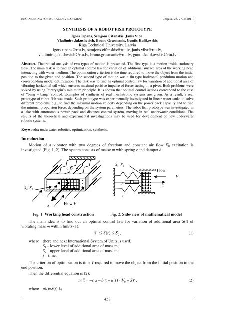
Introduction
Motion of a vibrator with two degrees of freedom and constant air flow ¯V 0 excitation is
investigated (Fig. 1, 2). The system consists of masse m with spring c and damper b.
c, b
S 1 , S 2
Flow
V
S 1 , S 2
b
x
c
x
Flow V
Fig. 1. Working head construction
458
Fig. 2. Side-view of mathematical model
The main idea is to find out an optimal control law for variation of additional area S(t) of
vibrating mass m within limits (1):
S
1
( S
2
where (here and next International System of Units is used)
S 1 – lower level of additional area of mass m;
S 2 – upper level of additional area of mass m;
t – time.
≤ S t)
≤ ,
(1)
The criterion of optimization is time T required to move the object from the initial position to the
end position.
Then the differential equation is (2):
where u(t)=S(t)·k;
m & x
= −c
x − b x&
− u( t)
⋅ ( V + x&
, (2)
2
0
)

ENGINEERING FOR RURAL DEVELOPMENT Jelgava, 26.-27.05.2011.
c – stiffness of spring;
b – damping coefficient;
V 0 – constant velocity of water;
S(t) – area variation;
u(t) – control action (2);
k – constant.
It is required to determine the control action u = u(t) for displacement of a system (2) from the
initial position x(t 0 ) to the end position x(t 1 ) in minimal time (criterion K) K=T, if the area S(t) has limit
(1).
Solution of optimal control problem for system with one degree of freedom
For system excitation any time the high-speed problem must be solved [1-3]:
t
K ∫1
⋅ dt
(3)
=
1
To assume t = ; t = , from (3) we have K = T .
0
0
1
T
t
The problems have been solved using the maximum principle of Pontryagin. It is find out that
optimal control action corresponds to the case of bound values of area limits S 1 , S 2 [4-9].
0
Real control action synthesis
For realizing optimal control actions (in general case) the system of one degree of freedom needs
a feedback system with two adapters: one for displacement measurement and another - for velocity
measurement. There is a simple case of control existing with only one adapter when motion changes
directions [2-4]. It means that the control action is similar to negative dry friction and switch points are
along zero velocity line. In that case equation of motion for large velocity V 0 ≥ x&
is (4):
where
m ⋅ & x
= −c
⋅ x − b ⋅ x&
+ U(x), &
(4)
⎡ 2 1+
sign(
x&
) ⎤ ⎡
2
U ( x&
) = −
⎢
k ⋅(
V0
+ x&
) ⋅ S1
⋅
⎥
−
⎢
k ⋅ ( V0
+ x&
) ⋅ S2
⎣
2 ⎦ ⎣
m – mass;
c, b, F, k, V 0 – constants.
Examples of modelling are shown in Fig. 3-4.
1−
sign(
x&
) ⎤
⋅
2 ⎥
⎦
Pa
-0.6
-0.8
-1
0 1 2
t n
3
2
1
0
-1
-2
v n
⎛ x
0 ⎞ ⎛2.3⎞
⎜
⎟ : = ⎜ ⎟
⎝ v0
⎠ ⎝ 0 ⎠
-3 -2.45 -2.4 -2.35 -2.3 -2.25
x n
Fig. 3. Full control action Pa n =U( x) ̇ in time t n
domain (SI system)
Fig. 4. Motion in phase plane (x=x n ; x=v ̇ n ) with
initial conditions inside of limit cycle
Optimization and synthesis of robot fish tail rotation motion
The second object of the theoretical study is a fin type propulsive device of robotic fish moving
inside water. The aim of the study is to find out an optimal control law for variation of additional area
459

ENGINEERING FOR RURAL DEVELOPMENT Jelgava, 26.-27.05.2011.
of the vibrating tail like horizontal pendulum, which ensures maximal positive impulse of motion
forces components acting on the tail parallel x axe (Fig. 5, 6).
Tail
z
y
Stop
y
Spring of pendulum
Ay
Stop
S 1 , S 2
x
ϕ
S 1 , S 2
Tail
Ax
x
Fig. 5. Side-view of robot fish tail like
horizontal pendulum
Fig. 6. Top-view of robot fish tail like
horizontal pendulum. Simplify model with
fixed pivot A
The problem has been solved using the maximum principle of Pontryagin. It is shown that the
optimal control action corresponds to the case of bound values of area limits.
The mathematical model of the system consists of rigid straight flat tail moving around the pivot
(Fig. 6). The area of the tail may be changed by control actions. For motion excitation moment
M(t,φ,ω) around the pivot must be added, where ω=dφ/dt – angular velocity of rigid tail. For more
resources of the system an additional rotational spring with stiffness c may be added (Fig. 6).
The main idea of this report is to find out an optimal control law for variation of additional area B(t) of
the vibrating tail within limits (5):
B ≤ ( ≤ B , (5)
1
B t)
where B 1 – lower level of additional area of tail;
B 2 – upper level of additional area of tail;
t – time.
The criterion of optimization is full reaction Ax* impulse in the pivot, acted to hull (indirect
reaction to tail, Fig. 6.):
T
2
K = −∫ Ax * ⋅dt
, (6)
0
required to move the object from one stop initial position (φ max; ̇φ=0) to the second stop end position
(φ min , ̇φ=0) in time T.
The differential equation of motion of the system with one degree of freedom (by use exchange of
moment of momentum around a fixed point A) is:
A
t
L
∫
( & ϕ ⋅ξ
)
2
J & ϕ
= M ( t,
ϕ,
& ϕ)
− c ⋅ϕ
− k ⋅ B ⋅ sign(
& ϕ ⋅ϕ)
⋅ ⋅ξ
⋅ dξ
, (7)
where J A – moment inertia tail mass against pivot point;
̈φ – angular acceleration of rigid body straight tail;
M(t,φ, ̇φ) – excitation moment of drive;
c – angular stiffness;
k t – constant coefficient;
B – area;
0
460

ENGINEERING FOR RURAL DEVELOPMENT Jelgava, 26.-27.05.2011.
(
L
∫
0
2
( ⋅ξ
) ⋅ξ
⋅ dξ )
ϕ& – component of moment of resistance force like integral along tail
direction;
̇φ – angular velocity;
L – length of the tail.
From theorem of tail mass m centre motion follows (8) (Fig. 6.):
⎛ 2 L
L ⎞
m ⋅ ⎜ & ϕ ⋅ ⋅ cosϕ
+ && ϕ ⋅ ⋅ sinϕ
⎟ = Ax − k
⎝ 2
2 ⎠
After integration from equations (6) and (7) we have (9, 10):
2 L 1
Ax = m ⋅{
& ϕ ⋅ ⋅ cos( ϕ)
+
2 J
t
⎛
⋅ B ⋅ sin( ϕ)
⋅ sign(
ϕ ⋅ & ϕ)
⋅ ⎜
⎝
L
∫
0
⎞
2
( & ϕ ⋅ξ
) ⋅ dξ
⎟ ⎠
4
1 ⎡
2 L ⎤
& ϕ
= ⋅ ⎢M
( t,
ϕ,
& ϕ)
− c ⋅ϕ
− k ⋅ B ⋅ sign(
&
t
ϕ)
⋅ & ϕ ⋅ ⎥
(9)
J
A ⎣
4 ⎦
3
2 L
+ kt
⋅ B ⋅ sin( ϕ)
⋅ sign(
ϕ ⋅ & ϕ)
⋅ & ϕ ⋅ .
3
A
⎡
⋅ ⎢M
( t,
ϕ,
& ϕ)
− c ⋅ϕ
− k
⎣
Then the criterion of optimization (fool impulse) is:
T
K = −∫
0
⎛
2 L 1 ⎡
⎜m
⋅{
& ϕ ⋅ ⋅ cos( ϕ)
+ ⋅ M ( t,
, ) c k
2 J
⎢ ϕ & ϕ − ⋅ϕ
−
t
⎜
A ⎣
⎜
3
⎜
2 L
+ kt
⋅ B ⋅sin(
ϕ)
⋅ sign(
ϕ ⋅ & ϕ)
⋅ & ϕ ⋅
⎝
3
t
(8)
4
2 L ⎤ L
⋅ B ⋅ sign(
& ϕ)
⋅ & ϕ ⋅ ⋅ ⋅ sin( )} +
4
⎥ ϕ
⎦ 2
(10)
4
2 L ⎤
⋅ B ⋅ sign(
& ϕ)
⋅ & ϕ ⋅
4
⎥ ⋅
⎦
L ⎞
⋅sin(
ϕ)}
+ ⎟
2 ⎟
⎟⋅
dt.
(11)
⎟
⎠
The last equations (11) can be used in the task of optimizations. The solution of optimal control
problem for the system with one degree of freedom (9) by using the maximum principle of Portryaing
may be found out from equations (6, 7) [6-10]. Like before, the control action is on the bounds
boundaries (5).
Synthesis of system with adaptive excitation and adaptive area control
In a case of adaptive excitation moment M may be used like a function of angular velocity in a
form [3; 9] M(t)=M0·sign(ω). The results of modelling are shown in Fig. 7-10.
ω n
0
0.5
0.25
0
-0.25
-0.5
-0.3 -0.15 0 0.15 0.3
Fig. 7. Tail angular motion in phase plane –
angular velocity as function of angle
ϕ n
ε n
4
2.6
1.3
0
-1.33
-2.67
-4
-0.3 -0.2 -0.1 0 0.1 0.2 0.3
ϕ n
Fig. 8. Angular acceleration of tail as
function of angle
461

ENGINEERING FOR RURAL DEVELOPMENT Jelgava, 26.-27.05.2011.
ε n
4
2
0
-2
-4
0 2.5 5 7.5 10
Fig. 9. Angular acceleration ε = ̈φ of tail in
time domain
t n
0.05
0.025
0
-0.025
-0.05
-0.075
Ax n
-0.1
0 1.67 3.33 5 6.67 8.33 10
Fig. 10. Impulse Ax(t) in time domain
A prototype of robot fish for experimental investigations was made (Fig. 11, 12). This prototype
was investigated in a linear water tank with different aims, for example: – find maximal motion
velocity depending on the power pack capacity; – find minimal propulsion force, depending on the
system parameters.
Additionally this prototype was investigated in a large storage lake with autonomy power pack
and distance control system, moving in real under water conditions with waves. The results of the
theoretical and experimental investigation may be used for inventions of new robotic systems.
t n
1 2 3
4 5 6
Fig. 11. Top-view of prototype
Fig. 12. Inside prototype there are:
1 – microcontroller; three actuators
(4 – for level, 5 – direction and 6 – velocity control);
2 – power supply; 3 – radio signal detector
Conclusions
Motion of robotic fish tail vibration by simplified interaction with water flow give very easy
equations of motion analysis. That allows solving the mathematical problem of area control
optimization and gives information for new systems synthesis. Control (exchange) of the object area
under water allows finding very efficient mechatronic systems. For realization of such systems
adapters and controllers must be used. For this reason very simple control action has solutions with
use of sign functions. It is shown that real tail vibration motion is very stable and gives satisfactory
real criterion in the hull contact point.
References
1. Lavendelis E. Synthesis of optimal vibro machines. Zinatne, Riga, 1970. 252. p. (in Russian).
2. Lavendelis E., Viba J. Individuality of Optimal Synthesis of vibro impact systems. Book:
“Vibrotechnics”. Kaunas. Vol. 3 (20), 1973. pp. 47-54. (in Russian).
3. Viba J. Optimization and synthesis of vibro impact systems. Zinatne, Riga, 1988. 253. p. (in
Russian).
462

ENGINEERING FOR RURAL DEVELOPMENT Jelgava, 26.-27.05.2011.
4. Lavendelis E., Viba J. Methods of optimal synthesis of strongly non – linear (impact) systems.
Scientific Proceedings of Riga Technical University. Mechanics. Volume 24. Riga, 2007. pp. 9-
15.
5. Boltyanskii V.G., Gamkrelidze R.V. and Pontryagin L.S.: On the Theory of Optimum Processes
(In Russian), Dokl. AN SSSR, 110, No. 1, 1956. pp. 7-10.
6. Boltyanskii V.G. Mathematical Methods of Optimal Control, Nauka, Moscow. 1969. 408. p. (in
Russian).
7. Sonneborn, L., Van Vleck F. The Bang-Bang Principle for Linear Control Systems, SIAM J.
Control 2, 1965, pp. 151-159.
8. Tipans I., Viba J., Fontaine J.G., Kruusmaa M., Megill W., Cifanskis S. Theory of robot fish
plane motion. Scientific Proceedings of Riga Technical University. Mechanics. Volume 31. Riga,
2009. pp. 8-18.
9. Kulikovskis G., Abele M., E. Kovals., Tipans I., Cifanskis S., Kruusmaa M., Fontaine J.G., Viba
J. Robotic fish tail motion excitation by adaptive control. Scientific Proceedings of Riga
Technical University. Mechanics. Volume 33. Riga, 2010. pp. 15-20.
463