Towards an experimental von Karman dynamo: numerical studies ...

More documents

Recommendations

Info

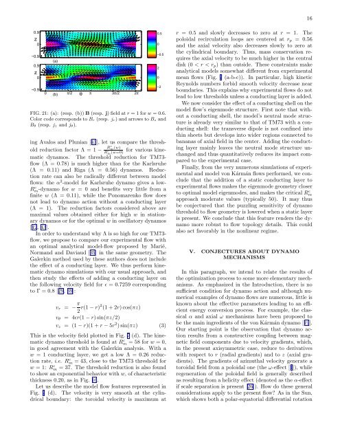
16 0.9 z 0 −0.9 0.9 z 0 −0.9 (a) θ 0 (b) π/2 π 3π/2 2π FIG. 21: (a): (resp. (b)) B (resp. j) field at r = 1 for w = 0.6. Color code corresponds to B r (resp. j r) and arrows to B z and B θ (resp. j z and j θ ). ing Avalos and Plunian [43], let us compare the threshold reduction factor Λ = 1 − Rc m (w) R c m (w=0) for various kinematic dynamos. The threshold reduction for TM73- flow (Λ = 0.78) is much higher than for the Karlsruhe (Λ = 0.11) and Riga (Λ = 0.56) dynamos. Reduction rate can also be radically different between model flows: the α 2 -model for Karlsruhe dynamo gives a low- Rm-dynamo c for w = 0 and benefits very little from a finite w (Λ = 0.11), while the Ponomarenko flow does not lead to dynamo action without a conducting layer (Λ = 1). The reduction factors considered above are maximal values obtained either for high w in stationary dynamos or for the optimal w in oscillatory dynamos [42, 43]. In order to understand why Λ is so high for our TM73- flow, we propose to compare our experimental flow with an optimal analytical model-flow proposed by Marié, Normand and Daviaud [39] in the same geometry. The Galerkin method used by these authors does not include the effect of a conducting layer. We thus perform kinematic dynamo simulations with our usual approach, and then study the effects of adding a conducting layer on the following velocity field for ǫ = 0.7259 corresponding to Γ = 0.8 [29, 39]: v r = − π 2 r(1 − r)2 (1 + 2r)cos(πz) 0.5 0 −0.5 v θ = 4ǫr(1 − r)sin(πz/2) v z = (1 − r)(1 + r − 5r 2 )sin(πz) (3) This is the velocity field plotted in Fig. 7 (d). The kinematic dynamo threshold is found at Rm c = 58 for w = 0, in good agreement with the Galerkin analysis. With a w = 1 conducting layer, we get a low Λ = 0.26 reduction rate, i.e. Rm c = 43, close to the TM73 threshold for w = 1: Rm c = 37. The threshold reduction is also found to show an exponential behavior with w, of characteristic thickness 0.20, as in Fig. 16. Let us describe the model flow features represented in Fig. 7 (d). The velocity is very smooth at the cylindrical boundary: the toroidal velocity is maximum at 2 0 −2 r = 0.5 and slowly decreases to zero at r = 1. The poloidal recirculation loops are centered at r p = 0.56 and the axial velocity also decreases slowly to zero at the cylindrical boundary. Thus, mass conservation requires the axial velocity to be much higher in the central disk (0 < r < r p ) than outside. These constraints make analytical models somewhat different from experimental mean flows (Fig. 7 (a-b-c)). In particular, high kinetic Reynolds numbers forbid smooth velocity decrease near boundaries. This explains why experimental flows do not lead to low thresholds unless a conducting layer is added. We now consider the effect of a conducting shell on the model flow’s eigenmode structure. First note that without a conducting shell, the model’s neutral mode structure is already very similar to that of TM73 with a conducting shell: the transverse dipole is not confined into thin sheets but develops into wider regions connected to bananas of axial field in the center. Adding the conducting layer mainly leaves the neutral mode structure unchanged and thus quantitatively reduces its impact compared to the experimental case. Finally, from the very numerous simulations of experimental and model von Kármán flows performed, we conclude that the addition of a static conducting layer to experimental flows makes the eigenmode geometry closer to optimal model eigenmodes, and makes the critical R c m approach moderate values (typically 50). It may thus be conjectured that the puzzling sensitivity of dynamo threshold to flow geometry is lowered when a static layer is present. We conclude that this feature renders the dynamo more robust to flow topology details. This could also act favorably in the nonlinear regime. V. CONJECTURES ABOUT DYNAMO MECHANISMS In this paragraph, we intend to relate the results of the optimization process to some more elementary mechanisms. As emphasized in the Introduction, there is no sufficient condition for dynamo action and although numerical examples of dynamo flows are numerous, little is known about the effective parameters leading to an efficient energy conversion process. For example, the classical α and axial ω mechanisms have been proposed to be the main ingredients of the von Kármán dynamo [19]. Our starting point is the observation that dynamo action results from a constructive coupling between magnetic field components due to velocity gradients, which, in the present axisymmetric case, reduce to derivatives with respect to r (radial gradients) and to z (axial gradients). The gradients of azimuthal velocity generate a toroidal field from a poloidal one (the ω-effect [1]), while regeneration of the poloidal field is generally described as resulting from a helicity effect (denoted as the α-effect if scale separation is present [26]). How do these general considerations apply to the present flow As in the Sun, which shows both a polar-equatorial differential rotation
17 and a tachocline transition, our experimental flow fields present azimuthal velocity shear in the axial and radial directions (see Fig. 2). We will therefore consider below the role of both the axial and the radial ω-effect. We will discuss these mechanisms and then suggest that, for a flow surrounded by a static conducting layer, the dynamo mechanism is based on the presence of a strong velocity shear (at the boundary layer r = 1) which lies in this case in the bulk of the overall electrically conducting domain. A. Axial ω-effect Induction simulations performed with the toroidal part of the velocity show an axial ω-effect which converts an imposed axial field into toroidal field through ∂v θ /∂z. Such a R m -linear effect has been demonstrated in the VKS1 experiment [20]. This effect is concentrated around the equatorial shear layer (z = 0) as visible in Fig. 2. Thus, we may surmise that the axial ω-effect is involved in the dynamo process: for dynamo action to take place, there is a need for another process to convert a toroidal magnetic field into a poloidal field. B. α-effect, helicity effect R m -non-linear conversion from transverse to axial magnetic field has also been reported in the VKS1 experiment [21]. This effect is not the usual scale-separation α-effect [26] and has been interpreted as an effect of the global helicity as reported by Parker [40] (in the following, it will be denoted “α”-effect). We believe it to take place in the high kinetic helicity regions of the flow (see Fig. 12). C. Is an “α”ω mechanism relevant Bourgoin et al. [46] performed a study of induction mechanisms in von Kármán-type flows, using a quasistatic iterative approach. They show that “α”ω dynamo action, seen as a three-step loop-back inductive mechanism, is possible, but very difficult to obtain, since fields are widely expelled by the vortices. The authors highlight the fact that the coupling between the axial ω-effect and the “α”-effect is very inefficient for our velocity fields, because of the spatial separation of these two induction effects. Our observations of the velocity and helicity fields confirm this separation. The authors also discovered an induction effect — the BC-effect — related to the magnetic diffusivity discontinuity at the insulating boundary that could be invoked in the dynamo mechanism. This BC-effect, illustrated on our TM73-velocity field (Fig. 14 in Ref. [46]), is enhanced in the case of strong velocity and vorticity gradients at the boundaries, characteristic of high Reynolds number flows. We are therefore convinced that for experimental flow fields at w = 0, the BC-effect helps the dynamo. This is consistant with our observations of high tangential current density near the boundaries and high magnetic energy production at r = 1 even for w = 0 (Fig. 19). Such a current sheet formation and BC-effect was reported by Bullard and Gubbins [24]. When a large layer of sodium at rest is added, the BCeffect vanishes because the conductivity discontinuity occurs at r = 1+w while the currents still are concentrated at the flow boundary r = 1. However, with a conducting layer, we have presented many features favoring the dynamo. In the next paragraph, we propose a possible origin for this conducting-layer effect. D. Radial ω-effect, boundary layers and static shell With a layer of steady conducting material surrounding the flow, we note the occurrence of two major phenomena: • the possibility for currents to flow freely in this shell (Fig. 19), • the presence of a very strong velocity shear localized at the boundary layer which now lies in the bulk of the electrically conducting domain. Let us again consider the shape of the velocity shear. Any realistic (with real hydrodynamical boundary conditions) von Kármán flow obviously presents negative gradients of azimuthal velocity ∂v θ /∂r between the region of maximal velocity and the flow boundary. This region can be divided into two parts: a smooth decrease in the bulk (R r 1) and a sharp gradient in the boundary layer at r = 1 (Fig. 7). These gradients are responsible for a radial ω-effect, producing B θ with B r , in both insulating and conducting cases. However, without a conducting layer, only the smooth part of the gradient which lies in the bulk will be efficient for dynamo action. Indeed, owing to the huge value of the kinetic Reynolds number and the very small value of the magnetic Prandtl number, the sharp boundary layer gradient is confined to a tiny domain, much smaller than the magnetic variation scale. No significant electrical currents can flow in it and we did not resolve this boundary layer with the numerical code: it is totally neglected by our approach. The role of both types of gradients is illustrated by the observation (Fig. 7 (c)) of impellers of large radius (R = 0.925). For such impellers there is almost no departure from solid body rotation profiles in the flow region and these impellers lead to dynamo action only with conducting shell [22], i.e., due to the sharp gradient. On the other hand, our R = 0.75 selected impellers present a stronger bulk-gradient and achieve dynamo in both cases (Fig. 7 (b)). In fact, the way we numerically modelized the von Kármán flow surrounded by a static conducting layer
Page 1 and 2: Towards an experimental von Kármá
Page 3 and 4: 3 Na at rest Liquid Na f -f R w c R
Page 5 and 6: 5 C. Global quantities and scaling
Page 7 and 8: 7 0 ing layer, we must look for the
Page 9 and 10: 9 Impeller α( 0 ) 〈P 〉〈T
Page 11 and 12: 11 IV. IMPACT OF A CONDUCTING LAYER
Page 13 and 14: 13 Rm c 200 150 100 50 0 0 0.2 0.4
Page 15: D. Neutral mode structure 5 0.16 (1
Page 19 and 20: 19 of a homogeneous two-scale dynam

Towards an experimental von Karman dynamo: numerical studies ...

You also want an ePaper? Increase the reach of your titles

Delete template?

Save as template?