Towards an experimental von Karman dynamo: numerical studies ...

Towards an experimental von Kármán dynamo: numerical studies for an optimized
design
Florent Ravelet, Arnaud Chiffaudel, ∗ and François Daviaud
Service de Physique de l’État Condensé, DSM, CEA Saclay, CNRS URA 2464, 91191 Gif-sur-Yvette, France
Jacques Léorat †
LUTH, Observatoire de Paris-Meudon, 92195 Meudon, France
(To be published in Phys. Fluids: August 25, 2005)
Numerical studies of a kinematic dynamo based on von Kármán type flows between two counterrotating
disks in a finite cylinder are reported. The flow has been optimized using a water model
experiment, varying the driving impellers’ configuration. A solution leading to dynamo action for
the mean flow has been found. This solution may be achieved in VKS2, the new sodium experiment
to be performed in Cadarache, France. The optimization process is described and discussed; then
the effects of adding a stationary conducting layer around the flow on the threshold, on the shape
of the neutral mode and on the magnetic energy balance are studied. Finally, the possible processes
involved in kinematic dynamo action in a von Kármán flow are reviewed and discussed. Among the
possible processes, we highlight the joint effect of the boundary-layer radial velocity shear and of
the Ohmic dissipation localized at the flow/outer-shell boundary.
ccsd-00003337, version 3 - 25 Aug 2005
PACS numbers: 47.65+a, 91.25.Cw
I. INTRODUCTION
In an electrically conducting fluid, kinetic energy can
be converted into magnetic energy, if the flow is both of
adequate topology and sufficient strength. This problem
is known as the dynamo problem [1], and is a magnetic
seed-field instability. The equation describing the behavior
of the magnetic induction field B in a fluid of resistivity
η under the action of a velocity field v is writen in
a dimensionless form:
∂B
∂t
= ∇ × (v × B) +
η
V ∗ L ∗ ∇2 B (1)
where L ∗ is a typical length scale and V ∗ a typical velocity
scale. In addition, one must take into account the
divergence-free nature of B, the electromagnetic boundary
conditions and the Navier-Stokes equations governing
the fluid motion, including the back-reaction of the
magnetic field on the flow through the Lorentz force.
The magnetic Reynolds number R m = V ∗ L ∗ η −1 ,
which compares the advection to the Ohmic diffusion,
controls the instability. Although this problem is simple
to set, it is still open. While some flows lead to the
dynamo instability with a certain threshold R c m, other
flows do not, and anti-dynamo theorems are not sufficient
to explain this sensitivity to flow geometry [1]. The
two recent experimental success of Karlsruhe and Riga
[2, 3, 4, 5, 6] are in good agreement with analytical and
numerical calculations [7, 8, 9, 10]; these two dynamos
belong to the category of constrained dynamos: the flow
∗ Electronic address: arnaud.chiffaudel@cea.fr
† Electronic address: Jacques.Leorat@obspm.fr
is forced in pipes and the level of turbulence remains low.
However, the saturation mechanisms of a dynamo are not
well known, and the role of turbulence on this instability
remains misunderstood [11, 12, 13, 14, 15, 16, 17].
The next generation of experimental homogeneous unconstrained
dynamos (still in progress, see for example
Frick et al., Shew et al., Marié et al. and O’Connell et
al. in the Cargèse 2000 workshop proceedings [18]) might
provide answers to these questions. The VKS liquidsodium
experiment in Cadarache, France [19, 20, 21] belongs
to this category. The VKS experiment is based on a
class of flows called von Kármán type flows. In a closed
cylinder, the fluid is inertially set into motion by two
coaxial counterrotating impellers fitted with blades. This
paper being devoted to the hydrodynamical and magnetohydrodynamical
properties of the mean flow, let us
first describe briefly the phenomenology of such mean
flow. Each impeller acts as a centrifugal pump: the
fluid rotates with the impeller and is expelled radially
by the centrifugal effect. To ensure mass conservation
the fluid is pumped in the center of the impeller and
recirculates near the cylinder wall. In the exact counterrotating
regime, the mean flow is divided into two toric
cells separated by an azimuthal shear layer. Such a mean
flow has the following features, known to favor dynamo
action: differential rotation, lack of mirror symmetry and
the presence of a hyperbolic stagnation point in the center
of the volume. In the VKS experimental devices,
the flow, inertially driven at kinetic Reynolds number up
to 10 7 (see below), is highly turbulent. As far as full
numerical MHD treatment of realistic inertially driven
high-Reynolds-number flows cannot be carried out, this
study is restricted to the kinematic dynamo capability of
von Kármán mean flows.
Several measurements of induced fields have been performed
in the first VKS device (VKS1) [20], in rather

2
good agreement with previous numerical studies [22], but
no dynamo was seen: in fact the achievable magnetic
Reynolds number in the VKS1 experiment remained below
the threshold calculated by Marié et al. [22]. A
larger device —VKS2, with diameter 0.6 m and 300 kW
power supply— is under construction. The main generic
properties of mean-flow dynamo action have been highlighted
by Marié et al. [22] on two different experimental
von Kármán velocity fields. Furthermore, various numerical
studies in comparable spherical flows confirmed the
strong effect of flow topology on dynamo action [23, 28].
In the experimental approach, many parameters can be
varied, such as the impellers’ blade design, in order to
modify the flow features. In addition, following Bullard
& Gubbins [24], several studies suggest adding a layer
of stationary conductor around the flow to help the dynamo
action. All these considerations lead us to consider
the implementation of a static conducting layer in the
VKS2 device and to perform a careful optimization of
the mean velocity field by a kinematic approach of the
dynamo problem.
Looking further towards the actual VKS2 experiment,
one should discuss the major remaining physical unexplored
feature: the role of hydrodynamical turbulence.
Turbulence in an inertially-driven closed flow will be very
far from homogeneity and isotropy. The presence of hydrodynamical
small scale turbulence could act in two different
ways: on the one hand, it may increase the effective
magnetic diffusivity, inhibiting the dynamo action [25].
On the other hand, it could help the dynamo through
a small-scale α-effect [26]. Moreover, the presence of a
turbulent mixing layer between the two counterrotating
cells may move the instantaneous velocity field away from
the time-averaged velocity field for large time-scales [27].
As the VKS2 experiment is designed to operate above
the predicted kinematic threshold presented in this paper,
it is expected to give an experimental answer to this
question of the role of turbulence on the instability. Furthermore,
if it exhibits dynamo action, it will shed light
on the dynamical saturation regime which is outside the
scope of the present paper.
In this article, we report the optimization of the timeaveraged
flow in a von Kármán liquid sodium experiment.
We design a solution which can be experimentally
achieved in VKS2, the new device held in Cadarache,
France. This solution particularly relies on the addition
of a static conducting layer surrounding the flow.
The paper is organized as follows. In Section II we first
present the experimental and numerical techniques that
have been used. In Section III, we present an overview of
the optimization process which lead to the experimental
configuration chosen for the VKS2 device. We study the
influence of the shape of the impellers both on the hydrodynamical
flow properties and on the onset of kinematic
dynamo action. In Section IV, we focus on the
understanding of the observed kinematic dynamo from a
magnetohydrodynamical point of view: we examine the
structure of the eigenmode and the effects of an outer
conducting boundary. Finally, in Section V, we review
some possible mechanisms leading to kinematic dynamo
action in a von Kármán flow and propose some conjectural
explanations based on our observations.
II.
EXPERIMENTAL AND NUMERICAL
TOOLS
A. What can be done numerically
The bearing of numerical simulations in the design of
experimental fluid dynamos deserves some general comments.
Kinetic Reynolds numbers of these liquid sodium
flows are typically 10 7 , well beyond any conceivable direct
numerical simulation. Moreover, to describe effective
MHD features, it would be necessary to treat very
small magnetic Prandtl numbers, close to 10 −5 , a value
presently not within computational feasibility. Several
groups are progressing in this way on model flows, for example
with Large Eddy Simulations [15] which can reach
magnetic Prandtl numbers as low as 10 −2 – 10 −3 . Another
strong difficulty arises from the search of realistic
magnetic boundary conditions treatment which prove in
practice also to be difficult to implement, except for the
spherical geometry.
An alternative numerical approach is to introduce a
given flow in the magnetic induction equation (1) and to
perform kinematic dynamo computations. This flow can
be either analytical [8, 23], computed by pure hydrodynamical
simulations (which may now be performed with
Reynolds numbers up to a few thousands), or measured
in laboratory water models [22, 28] by Laser Doppler
velocimetry (LDV) or by Particle Imaging Velocimetry
(PIV). Such measurements lead to a map of the timeaveraged
flow and to the main properties of the fluctuating
components: turbulence level, correlation times, etc.
Kinematic dynamo computations have been successfully
used to describe or to optimize the Riga [7] and Karlsruhe
[8] dynamo experiments.
We will follow here the kinematic approach using the
time-averaged flow measured in a water model at realistic
kinetic Reynolds number. Indeed, potentially important
features such as velocity fluctuations will not be
considered. Another strong limitation of the kinematic
approach is its linearity: computations may predict if an
initial seed field grows, but the study of the saturation
regime will rely exclusively on the results of the actual
MHD VKS-experiment.
B. Experimental measurements
In order to measure the time-averaged velocity field
—hereafter simply denoted as the mean field— we use
a water-model experiment which is a half-scale model of
the VKS2 sodium device. The experimental setup, measurement
techniques, and methods are presented in detail

3
Na at rest
Liquid Na
f -f
R w
c
R
c
1
H
c
r/R
0
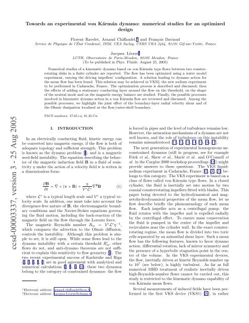
FIG. 1: Sketch of the VKS2 experiment. The container radius
R c is taken as unit scale. w is the dimensionless thickness of
sodium at rest.
in Refs. [22, 29]. However, we present below an overview
of our experimental issues and highlight the evolutions
with respect to those previous works.
We use water as the working fluid for our study, noting
that its hydrodynamical properties at 50 o C (kinematic
viscosity ν and density ρ) are very close to those
of sodium at 120 o C.
A sketch of the von Kármán experiments is presented
in Fig. 1. The cylinder is of radius R c and height
H c = 1.8R c . In the following, all the spatial quantities
are given in units of R c = L ∗ . The hydrodynamical
time scale is based on the impeller driving frequency
f: if V is the measured velocity field for a driving frequency
f, the dimensionless mean velocity field is thus
v = (2πR c f) −1 V.
The integral kinetic Reynolds number Re is typically
10 6 in the water-model, and 10 7 in the sodium device
VKS2. The inertially driven flow is highly turbulent,
with velocity fluctuations up to 40 percent of the maximum
velocity [20, 22]. In the water model, we measure
the time-averaged velocity field by Laser Doppler Velocimetry
(LDV). Data are averaged over typically 300
disk rotation periods. We have performed velocity measurements
at several points for several driving frequencies:
as expected for so highly turbulent a flow, the dimensionless
velocity v does not depend on the integral
Reynolds number Re = V ∗ L ∗ ν −1 [30].
Velocity modulations at the blade frequency have been
observed only in and very close to the inter-blade domains.
These modulations are thus time-averaged and
we can consider the mean flow as a solenoidal axisymmetric
vector field [31]. So the toroidal part of the velocity
field V θ (in cylindrical coordinates) and the poloidal
part (V z , V r ) are independent.
In the water-model experiment dedicated to the study
reported in this paper, special care has been given to
the measurements of velocity fields, especially near the
blades and at the cylinder wall, where the measurement
grid has been refined. The mechanical quality of the
experimental setup ensures good symmetry of the mean
velocity fields with respect to rotation of π around any
diameter passing through the center of the cylinder (R π -
1
−0.9 0 0.9
z/R
FIG. 2: Dimensionless mean velocity field measured by LDV
and symmetrized for kinematic dynamo simulations. The
cylinder axis is horizontal. Arrows correspond to poloidal
part of the flow, shading to toroidal part. We use cylindrical
coordinates (r, θ, z), with origin at the center of the cylinder.
symmetry). The fields presented in this paper are thus
symmetrized by R π with no noticeable changes in the
profiles but with a slightly improved spatial signal-tonoise
ratio. With respect to Ref. [22], the velocity fields
are neither smoothed, nor stretched to different aspect
ratios.
Fig. 2 shows the mean flow produced by the optimal
impeller. The mean flow respects the phenomenology
given in the Introduction: it is composed of two toroidal
cells separated by a shear layer, and two poloidal recirculation
cells. High velocities are measured over the
whole volume: the inertial stirring is actually very efficient.
Typically, the average over the flow volume of the
mean velocity field is of order of 0.3 × (2πR c f).
In addition to velocity measurements, we perform
global power consumption measurements: torques are
measured through the current consumption in the motors
given by the servo drives and have been calibrated
by calorimetry.
C. Kinematic dynamo simulations
Once we know the time-averaged velocity field, we integrate
the induction equation using an axially periodic
kinematic dynamo code, written by J. Léorat [32]. The
code is pseudo-spectral in the axial and azimuthal directions
while the radial dependence is treated by a highorder
finite difference scheme. The numerical resolution

4
corresponds to a grid of 48 points in the axial direction, 4
points in the azimuthal direction (corresponding to wave
numbers m = 0, ±1) and 51 points in the radial direction
for the flow domain. This spatial grid is the common basis
of our simulations and has been refined in some cases.
The time scheme is second-order Adams-Bashforth with
diffusive time unit t d = R 2 cη −1 . The typical time step is
5 ×10 −6 and simulations are generally carried out over 1
time unit.
Electrical conductivity and magnetic permeability are
homogeneous and the external medium is insulating. Implementation
of the magnetic boundary conditions for a
finite cylinder is difficult, due to the non-local character
of the continuity conditions at the boundary of the
conducting fluid. In contrast, axially periodic boundary
conditions are easily formulated, since the harmonic external
field then has an analytical expression. We thus
choose to look for axially periodic solutions, using a relatively
fast code, which allows us to perform parametric
studies. To validate our choice, we compared our results
with results from a finite cylinder code (F. Stefani,
private communication) for some model flows and a few
experimental flows. In all these cases, the periodic and
the finite cylinder computations give comparable results.
This remarkable agreement may be due to the peculiar
flow and to the magnetic eigenmodes symmetries: we do
not claim that it may be generalized to other flow geometries.
Indeed, the numerical elementary box consists
of two mirror-symmetric experimental velocity fields in
order to avoid strong velocity discontinuities along the z
axis. The magnetic eigenmode could be either symmetric
or antisymmetric with respect to this artificial mirror
symmetry [33]. In almost all of our simulations, the magnetic
field is mirror-antisymmetric, and we verify that no
axial currents cross the mirror boundary. The few exotic
symmetric cases we encountered cannot be used for
optimization of the experiment.
Further details on the code can be found in Ref. [32].
We use a mirror-antisymmetric initial magnetic seed field
optimized for a fast transient [22]. Finally, we can act
on the electromagnetic boundary conditions by adding
a layer of stationary conductor of dimensionless thickness
w, surrounding the flow exactly as in the experiment
(Fig. 1). This extension is made while keeping the grid
radial resolution constant (51 points in the flow region).
The velocity field we use as input for the numerical simulations
is thus simply in an homogeneous conducting
cylinder of radius 1 + w:
III.
OPTIMIZATION OF THE VKS
EXPERIMENT
A. Optimization process
The goal of our optimization process is to find the impeller
whose mean velocity field leads to the lowest R c m
for the lowest power cost. We have to find a solution feasible
in VKS2, i.e. with liquid sodium in a 0.6 m diameter
cylinder with 300 kW power supply. We performed an
iterative optimization loop: for a given configuration, we
measure the mean velocity field and the power consumption.
Then we simulate the kinematic dynamo problem.
We try to identify features favoring dynamo action and
modify parameters in order to reduce the threshold and
the power consumption and go back to the loop.
B. Impeller tunable parameters.
The impellers are flat disks of radius R fitted with 8
blades of height h. The blades are arcs of circles, with
a curvature radius C, whose tangents are radial at the
center of the disks. We use the angle α = arcsin( R
2C ) to
label the different curvatures (see Fig. 3). For straight
blades α = 0. By convention, we use positive values to
label the direction corresponding to the case where the
fluid is set into motion by the convex face of the blades.
In order to study the opposite curvature (α < 0) we
just rotate the impeller in the other direction. The two
counterrotating impellers are separated by H c , the height
of the cylinder. We fixed the aspect ratio H c /R c of the
flow volume to 1.8 as in the VKS device. In practice
we successively examine the effects of each parameter h,
R and α on global quantities characterizing the mean
flow. We then varied the parameters one by one, until we
found a relative optimum for the dynamo threshold. We
tested 12 different impellers, named TMxx, with three
radii (R = 0.5, 0.75 & 0.925), various curvature angles α
and different blade heights h.
+
R
α
v ≡ v measured for 0 ≤ r ≤ 1
v ≡ 0 for 1 < r ≤ 1 + w
FIG. 3: Sketch of the impeller parameters. R is the dimensionless
radius, α the blade curvature angle. The sign of α
is determined by the sense of rotation: positive when rotated
anticlockwise.

5
C. Global quantities and scaling relations
2.5
We know from empirical results [22, 23, 28] that the
poloidal to toroidal ratio Γ of the flow has a great impact
on the dynamo threshold. Moreover, a purely toroidal
flow is unable to sustain dynamo action [34, 35], while
it is possible for a purely poloidal flow [36, 37]. We also
note that, for a Ponomarenko flow, the pitch parameter
plays a major role [7, 16, 17]. All these results lead us to
first focus on the ratio
Γ = 〈P 〉
〈T 〉
0
−90 −45 0 45 90
where 〈P 〉 is the spatially averaged value of the poloidal
α
part of the mean flow, and 〈T 〉 the average of the toroidal
part.
Another quantity of interest is the velocity factor V: FIG. 4: MaDo number vs α for all the impellers we have
the dimensionless maximum value of the velocity. In our tested. R = 0.925(), R = 0.75() and R = 0.5(•). Closed
symbols: h = 0.2. Open symbols: h ≤ 0.1
simulations, the magnetic Reynolds number R m is based
on the velocity factor, i.e. on a typical measured velocity
in order to take into account the stirring efficiency:
This means that we have to look both at the global hydrodynamical
quantities and at the magnetic induction
V = max(||V||)
stability when varying the impellers’ tunable parameters
2 π R c f
h, R and α.
Fig. 4 presents MaDo for the entire set of impellers.
R m = 2 π R 2 c f V / η
For our class of impellers, the MaDo number remains of
the same order of magnitude within ±10%. Only the
We also define a power coefficient K p by dimensional smallest diameter impeller (R = 0.5) exhibits a slightly
analysis. We write the power P given by a motor to higher value. In the ideal case of homogeneous isotropic
sustain the flow as follows:
turbulence, far from boundaries, we can show that what
we call the MaDo number is related to the Kolmogorov
P = K p (Re, geometry)ρ Rc 5 Ω3
constant C K ≃ 1.5 [38]. The Kolmogorov constant is
related to the kinetic energy spatial spectrum:
with ρ the density of the fluid and Ω = 2πf the driving
pulsation. We have checked [29] that K p does not depend
on the Reynolds number Re as expected for so highly
E(k) = C K ǫ 2/3 k −5/3
turbulent inertially driven flows [30].
The velocity factor measures the stirring efficiency: the where ǫ is the dissipated power per unit mass, and k the
greater V, the lower the rotation frequency needed to wave number. If we assume that ǫ is homogeneous and
reach a given velocity. Besides, a lower K p implies that that P is the total dissipated power we measure, we have:
less power is needed to sustain a given driving frequency.
P
The dimensionless number which we need to focus on
ǫ =
compares the velocity effectively reached in the flow to
ρπRc 2H c
the power consumption. We call it the MaDo number: Using the definition
MaDo =
V
∫
1
K 1/3
p
2 〈v2 〉 = E(k)dk
The greater MaDo, the less power needed to reach a given and assuming 1 2 〈v2 〉 ≃ 1 2 V2 and using the steepness of
velocity (i.e. a given magnetic Reynolds number). The the spectrum, we obtain:
MaDo number is thus a hydrodynamical efficiency coefficient.
To make the VKS experiment feasible at laboratory
scale, it is necessary both to have great MaDo num-
E(k 0 ) = 1 3 V2 k0
−1
bers and low critical magnetic Reynolds numbers Rm c . with k 0 = 2π/R c the injection scale. Then the relation
The question underlying the process of optimization is between the MaDo number and C K is:
to know if we can, on the one hand, find a class of impellers
with mean flows exhibiting dynamo action, and,
( ) −2/3
on the other hand, if we can increase the ratio MaDo/Rm c . MaDo 2 ≃ 3π −4/3 Hc
C K ≃ 0.44 C K
R c
MaDo
2
1.5
1
0.5

6
i.e., with C K = 1.5, we should have, for homogeneous
isotropic turbulence MaDo ≃ 0.81. In our closed system
with blades, we recover the same order of magnitude,
and the fact that MaDo is almost independent of the
driving system. Thus, there is no obvious optimum for
the hydrodynamical efficiency. Between various impellers
producing dynamo action, the choice will be dominated
by the value of the threshold R c m .
Let us first eliminate the effect of the blade height h.
The power factor K p varies quasi-linearly with h. As
MaDo is almost constant, smaller h impellers require
higher rotation frequencies, increasing the technical difficulties.
We choose h = 0.2, a compromise between stirring
efficiency and the necessity to keep the free volume
sufficiently large.
σ
0
−5
−10
−15
Tm71
Tm73
−20
0.5 0.6 0.7 0.8 0.9 1
Γ
D. Influence of the poloidal/toroidal ratio Γ
In our cylindrical von Kármán flow without a conducting
layer (w = 0), there seems to be an optimal value for
Γ close to 0.7. Since the mean flow is axisymmetric and
divergence-free, the ratio Γ can be changed numerically
by introducing an arbitrary multiplicative factor on, say,
the toroidal part of the velocity field. In the following, Γ 0
stands for the experimental ratio for the measured mean
velocity field v exp , whereas Γ stands for a numerically
adjusted velocity field v adj . This flow is simply adjusted
as follows:
⎧
⎨
⎩
v adj
vr
adj
θ
= v exp
θ
= (Γ/Γ 0 ) · vr
exp
v adj
z
= (Γ/Γ 0 ) · v exp
z
In Fig. 5, we plot the magnetic energy growth rate σ
(twice the magnetic field growth rate) for different values
of Γ, for magnetic Reynolds number R m = 100 and
without conducting layer (w = 0). The two curves correspond
to two different mean velocity fields which have
been experimentally measured in the water model (they
correspond to the TM71 and TM73 impellers, see table I
for their characteristics). We notice that the curves show
the same shape with maximum growth rate at Γ ≃ 0.7,
which confirms the results of Ref. [22].
For Γ 0.6, oscillating damped regimes (open symbols
in Fig. 5) are observed. We plot the temporal evolution of
the magnetic energy in the corresponding case in Fig. 6:
these regimes are qualitatively different from the oscillating
regimes already found in [22] for non R π -symmetric
Γ = 0.7 velocity fields, consisting of one mode with a
complex growth rate: the magnetic field is a single traveling
wave, and the magnetic energy, integrated over the
volume, evolves monotonically in time.
In our case, the velocity field is axisymmetric and R π -
symmetric, i.e., corresponds to the group O(2) [33]. The
evolution operator for the magnetic field also respects
these symmetries. It is known that symmetries strongly
constrain the nature of eigenvalues and eigenmodes of
FIG. 5: Magnetic energy growth rate σ vs. numerical ratio Γ.
R m = 100, w = 0. Simulations performed for two different
mean velocity fields (impellers TM71 () and TM73 () of
radius R = 0.75). Larger symbols correspond to natural Γ 0 of
the impeller. Vertical dashed line corresponds to optimal Γ =
0.7. Closed symbols stand for stationary regimes, whereas
open symbols stand for oscillating regimes for Γ 0.6.
linear stability problems. We observe two types of nonaxisymmetric
m = 1 solutions consistent with the O(2)
group properties:
• A steady bifurcation with a real eigenvalue. The
eigenmode is R π -symmetric with respect to a certain
axis. We always observed such stationary
regimes for Γ 0.6.
• Oscillatory solutions in the shape of standing waves
associated with complex-conjugate eigenvalues.
The latter oscillatory solutions are observed for Γ
0.6. Since the temporal integration starts with a R π -
symmetric initial condition for the magnetic field, we obtain
decaying standing waves corresponding to the sum of
two modes with complex-conjugate eigenvalues and the
same amplitudes. The magnetic energy therefore decays
exponentially while pulsating (Fig. 6 (a)).
The same feature has been reported for analytical
“s 0 2t 0 2 − like flows” in a cylindrical geometry with a
Galerkin analysis of neutral modes and eigenvalues for
the induction equation [39]. A major interest of the latter
method is that it gives the structure of the modes: one
mode is localized near one impeller and rotates with it,
the other is localized and rotates with the other impeller.
Growing oscillating dynamos are rare in our system: a
single case has been observed, for TM71(−) (Γ 0 = 0.53)
with a w = 0.4 conducting layer at R m = 215 (R c m = 197,
see table I). Such high a value for the magnetic Reynolds
number is out of the scope of our experimental study, and
is close to the practical upper limit of the numerical code.
Experimental dynamo action will thus be sought in the
stationary regimes domain Γ 0.6. Without a conduct-

7
0
ing layer, we must look for the optimal impeller around
Γ 0 ≃ 0.7.
E. Effects of the impeller radius R
log (E)
−5
1
0.5
R=0.5
(a)
(e)
V θ
V z
−10
(a)
0 0.2 0.4 0.6 0.8 1
time
0.6
0
0 0.25 r 0.75 1
1
R=0.75
(b)
−0.5
0 0.25 r 0.75 1
0.5
(f)
0.4
V θ
V z
B z
0.2
0
−0.2
0
0 0.25 r 0.75 1
1
R=0.925
(c)
−0.5
0 0.25 r 0.75 1
0.5
(g)
−0.4
V θ
V z
(b)
−0.6
0 0.2 0.4 0.6 0.8 1
time
FIG. 6: Typical damped oscillating regime for impeller TM70
at Γ = 0.5, w = 0, R m = 140. (a): temporal evolution of the
magnetic energy E = ∫ B 2 . Straight line is a linear fit of the
form E(t) = E 0 exp(σt) and gives the temporal growth rate
σ = −12.1. (b): temporal evolution of the z component of
B at the point r = 0.4, θ = 0, z = −0.23 with a nonlinear fit
of the form: B z(t) = a exp(σt/2) cos(ωt + φ) which gives
σ = −12.2 and ω = 20.7.
V θ
0
0 0.25 r 0.75 1
1
Model
(d)
0
0 0.25 r 0.75 1
−0.5
0 0.25 r 0.75 1
0.5
V z
(h)
−0.5
0 0.25 r 0.75 1
FIG. 7: Radial profiles of toroidal velocity v θ ((a)–(d)) for z =
0.3 (dotted line), 0.675 (dashed line), & 0.9 (solid line); and
axial velocity v z ((e)–(h)) for various equidistant z between
the two rotating disks. From top to bottom: experimental
flow for (a-e): R = 0.5, (b-f): R = 0.75, (c-g): R = 0.925
impeller and (d-h): model analytical flow (see equations (3)
and discussion below).
One could a priori expect that a very large impeller
is favorable to the hydrodynamical efficiency. This is
not the case. For impellers with straight blades, MaDo
slightly decreases with R: for respectively R = 0.5, 0.75
and 0.925, we respectively get MaDo = 2.13, 1.64 and
1.62. This tendency is below the experimental error. We
thus consider that MaDo does not depend on the impeller.
Nevertheless one should not forget that V varies quasilinearly
with impeller radius R: if the impeller becomes
smaller it must rotate faster to achieve a given value for
the magnetic Reynolds number, which may again cause

8
mechanical difficulties. We do not explore radii R smaller
than 0.5.
Concerning the topology of the mean flow, there are
no noticeable effects of the radius R on the poloidal part.
We always have two toric recirculation cells, centered at
a radius r p close to 0.75±0.02 and almost constant for all
impellers (Fig. 7 (e-f-g-h)). The fluid is pumped to the
impellers for 0 < r < r p and is reinjected in the volume
r p < r < 1. This can be interpreted as a geometrical
constraint to ensure mass conservation: the circle of radius
r = √ 2
2
(very close to 0.75) separates the unit disk
into two regions of the same area.
The topology of the toroidal part of the mean flow now
depends on the radius of the impeller. The radial profile
of v θ shows stronger departure from solid-body rotation
for smaller R (Fig. 7 (a-b-c-d)): this will be emphasized
in the discussion. We performed simulations for three
straight blades impellers of radii R = 0.5, R = 0.75 and
R = 0.925; without a conducting shell (w = 0) and with
a conducting layer of thickness w = 0.4. We have integrated
the induction equation for the three velocity fields
numerically set to various Γ and compared the growth
rates. The impeller of radius R = 0.75 close to the radius
of the center of the poloidal recirculation cells systematically
yields the greatest growth rate. Thus, radius
R = 0.75 has been chosen for further investigations.
Γ 0
1
0.8
0.6
0.4
0.2
0
−45 −30 −15 0 15 30 45
α
FIG. 8: Γ 0 vs α for four impellers of radius R = 0.75 rotated
in positive and negative direction (see Table I).
F. Search for the optimal blade curvature
The hydrodynamical characteristics of the impellers of
radius R = 0.75 are given in table I. For increasing blade
curvature the average value of the poloidal velocity 〈P 〉
increases while the average value of the toroidal velocity
〈T 〉 decreases: the ratio Γ 0 is a continuous growing
function of curvature α (Fig. 8). A phenomenological explanation
for the 〈T 〉 variation can be given. The fluid
pumped by the impeller is centrifugally expelled and is
constrained to follow the blades. Therefore, it exits the
impeller with a velocity almost tangent to the blade exit
angle α. Thus, for α < 0 (resp. α > 0), the azimuthal
velocity is bigger (resp. smaller) than the solid body rotation.
Finally, it is possible to adjust Γ 0 to a desired
value by choosing the appropriate curvature α, in order
to lower the threshold for dynamo action.
Without a conducting shell, the optimal impeller is the
TM71 (Γ 0 = 0.69). But its threshold R c m = 179 cannot
be achieved in the VKS2 experiment. We therefore must
find another way to reduce R c m, the only relevant factor
for the optimization.
G. Optimal configuration to be tested in the VKS2
sodium experiment
σ
20
10
0
−10
−20
0.5 0.6 0.7 0.8 0.9 1
Γ
FIG. 9: Shift in the optimal value of Γ when adding a conducting
layer. Magnetic energy growth rate σ vs. Γ for w = 0
(•) and w = 0.4 (). Impeller TM73, R m = 100. Larger
symbols mark the natural Γ 0 of the impeller.
As in the Riga experiment [4, 7], and as in numerical
studies of various flows [24, 42, 43], we consider a stationary
layer of fluid sodium surrounding the flow. This

9
Impeller α( 0 ) 〈P 〉 〈T 〉 Γ 0 = 〈P 〉
〈T 〉 〈P 〉.〈T 〉 〈H〉 V Kp MaDo Rc m (w = 0) R c m (w = 0.4)
TM74− −34 0.15 0.34 0.46 0.052 0.43 0.78 0.073 1.86 n.i. n.i.
TM73− −24 0.16 0.34 0.48 0.055 0.41 0.72 0.073 1.73 n.i. n.i.
TM71− −14 0.17 0.33 0.53 0.057 0.49 0.73 0.069 1.79 n.i. 197 (o)
TM70 0 0.18 0.30 0.60 0.056 0.47 0.65 0.061 1.64 (1) (1)
TM71 +14 0.19 0.28 0.69 0.053 0.44 0.64 0.056 1.66 179 51
TM73 +24 0.20 0.25 0.80 0.051 0.44 0.60 0.053 1.60 180 43
TM74 +34 0.21 0.24 0.89 0.050 0.44 0.58 0.043 1.65 ∞ 44
TABLE I: Global hydrodynamical dimensionless quantities (see text for definitions) for the radius R = 0.75 impeller family,
rotating counterclockwise (+), or clockwise (−) (see Fig. 3). The last two columns present the thresholds for kinematic dynamo
action with (w = 0.4) and without (w = 0) conducting layer. Optimal values appear in bold font. Most negative curvatures
have not been investigated (n.i.) but the TM71−, which presents an oscillatory (o) dynamo instability for R c m = 197 with
w = 0.4. (1): the TM70 impeller (Γ 0 = 0.60) has a tricky behavior, exchanging stability between steady modes, oscillatory
modes and a singular mode which is mirror-symmetric with respect to the periodization introduced along z and thus not
physically relevant.
σ
5
0
−5
−10
Tm70
Tm71
Tm73
Tm74
−15
0.5 0.6 0.7 0.8 0.9 1
Γ
In Fig. 11, we plot the growth rates σ of the magnetic
energy simulated for four experimentally measured
mean velocity fields at various R m and for w = 0.4. The
impeller TM73 was designed to create a mean velocity
field with Γ 0 = 0.80. It appears to be the best impeller,
with a critical magnetic Reynolds number of R c m = 43.
Its threshold is divided by a factor 4 when adding a
layer of stationary conductor. This configuration (TM73,
w = 0.4) will be the first one tested in the VKS2 experiment.
The VKS2 experiment will be able to reach the
threshold of kinematic dynamo action for the mean part
of the flow. Meanwhile, the turbulence level will be high
and could lead to a shift or even disappearance of the
kinematic dynamo threshold. In Section IV, we examine
in detail the effects of the boundary conditions on the
TM73 kinematic dynamo.
FIG. 10: Growth rate σ of magnetic energy vs numerical ratio
Γ. R m = 43, w = 0.4 for 4 different R = 0.75 impellers: TM70
(•), TM71 (), TM73 () and TM74 (◮). Larger symbols
mark the natural Γ 0 of each impeller.
significantly reduces the critical magnetic Reynolds number,
but also slightly shifts the optimal value for Γ. We
have varied w between w = 0 and w = 1; since the
experimental VKS2 device is of fixed overall size (diameter
0.6 m), the flow volume decreases while increasing
the static layer thickness w. A compromise between this
constraint and the effects of increasing w has been found
to be w = 0.4 and we mainly present here results concerning
this value of w. In Fig. 9, we compare the curves
obtained by numerical variation of the ratio Γ for the
same impeller at the same R m , in the case w = 0, and
w = 0.4. The growth rates are much higher for w = 0.4,
and the peak of the curve shifts from 0.7 to 0.8. We have
performed simulations for velocity fields achieved using
four different impellers (Fig. 10), for w = 0.4 at R m = 43:
the result is very robust, the four curves being very close.
H. Role of flow helicity vs. Poloidal/Toroidal ratio
Most large scale dynamos known are based on helical
flows [1, 40]. As a concrete example, while successfully
optimizing the Riga dynamo experiment, Stefani et al. [7]
noticed that the best flows were helicity maximizing. The
first point we focused on during our optimization process,
i.e., the existence of an optimal value for Γ, leads us to
address the question of the links between Γ and mean
helicity 〈H〉. In our case, for aspect ratio H c /R c = 1.8
and impellers of radius R = 0.75, the mean helicity at
a given rotation rate 〈H〉 = ∫ v.(∇ × v) rdrdz does not
depend on the blade curvature (see Table I). Observation
of Fig. 12 also reveals that the dominant contribution in
the helicity scalar product is the product of the toroidal
velocity (v θ ∝ 〈T 〉) by the poloidal recirculation cells
vorticity ((∇ × v) θ ∝ 〈P 〉). We can therefore assume
the scaling 〈H〉 ∝ 〈P 〉〈T 〉, which is consistent with the
fact that the product 〈P 〉〈T 〉 and 〈H〉 are both almost
constant (Table I).
To compare the helicity content of different flows, we

10
σ
20
Rm=150
15
Rm=107
10
Rm=64
5
0
Rm=43
−5
−10
Rm=21
−15
−20
0.5 0.6 0.7 Γ 0
0.8 0.9 1
now consider the mean helicity at a given R m , 〈H〉/V 2 ,
more relevant for the dynamo problem. Figure 13
presents 〈H〉/V 2 versus Γ 0 for all h = 0.2 impellers. The
R = 0.75 family reaches a maximum of order of 1 for
Γ 0 ≃ 0.9. This tendency is confirmed by the solid curve
which shows a numerical variation of Γ for the TM73
velocity field and is maximum for Γ = 1. In addition,
even though R = 0.925 impellers give reasonably high
values of helicity near Γ = 0.5, there is an abrupt break
in the tendency for high curvature: TM60 (see Ref. [22])
exhibits large Γ 0 = 0.9 but less helicity than TM74. Inset
in Fig. 13 highlights this optimum for 〈H〉/V 2 versus
impeller radius R. This confirms the impeller radius
R = 0.75 we have chosen during the optimization described
above.
FIG. 11: Growth rate σ vs natural ratio Γ 0 for five impellers
at various R m and w = 0.4. From left to right: TM71−
with Γ 0 = 0.53, TM70 (Γ 0 = 0.60), TM71 (Γ 0 = 0.69), TM73
(Γ 0 = 0.80), TM74 (Γ 0 = 0.89), see also table I). Closed symbols:
stationary modes. Open symbols: oscillating modes.
1.5
1
/V 2
1
0
0 0.5 1
R
0.5
0
0 0.2 0.4 0.6 0.8 1 1.2
Γ ,Γ 0
0.9
0.9
z
z
0
0
−0.9
−0.9
0
(a)
0.5 1 0
(b)
0.5 1
r
r
1.2
1.0
0.8
0.6
0.4
0.2
0.0
−0.2
−0.4
−0.6
FIG. 13: Mean helicity at a given R m (〈H〉/V 2 ) vs. poloidal
over toroidal ratio. The R = 0.75 impeller series () is plotted
as a function of Γ 0. The large open symbol stands for TM73
at Γ 0 and the solid line stands for the same quantity plotted
vs. numerical variation of TM73 velocity field (Γ). We also
plot 〈H〉/V 2 vs. Γ 0 for the R = 0.5 (⋆) and R = 0.925 (□)
impellers. The inset presents 〈H〉/V 2 vs. impeller radius R
for impellers of 0.8 Γ 0 0.9.
FIG. 12: Contours of kinetic helicity H = v.(∇×v) for TM73
velocity field. (a): total helicity. (b): azimuthal contribution
v θ .(∇ × v) θ is dominant.
Since the optimal value toward dynamo action for the
ratio Γ (close to 0.7 − 0.8, depending on w) is lower
than 1, the best velocity field is not absolutely helicitymaximizing.
In other words, the most dynamo promoting
flow contains more toroidal velocity than the helicitymaximizing
flow. As shown by Leprovost [41], one can
interpret the optimal Γ as a quantity that maximizes the
product of mean helicity by a measure of the ω-effect,
i.e., the product 〈H〉〈T 〉 ∼ 〈P 〉〈T 〉 2 .

11
IV. IMPACT OF A CONDUCTING LAYER ON
THE NEUTRAL MODE AND THE ENERGY
BALANCE FOR THE VKS2 OPTIMIZED
VELOCITY FIELD
In this section, we discuss the mean velocity field produced
between two counterrotating TM73 impellers in a
cylinder of aspect ratio Hc
R c
= 1.8, like the first experimental
configuration chosen for the VKS2 experiment. See
Table I for the characteristics of this impeller, and Fig. 2
for a plot of the mean velocity field. We detail the effects
of adding a static layer of conductor surrounding the flow
and compare the neutral mode structures, the magnetic
energy and spatial distribution of current density for this
kinematic dynamo.
A. Neutral mode for w = 0
Without a conducting layer, this flow exhibits dynamo
action with a critical magnetic Reynolds number Rm c =
180. The neutral mode is stationary in time and has an
m = 1 azimuthal dependency. In Fig. 14, we plot an isodensity
surface of the magnetic energy (50% of the maximum)
in the case w = 0 at R m = Rm c = 180. The field
is concentrated near the axis into two twisted bananashaped
regions of strong axial field. Near the interface
between the flow and the outer insulating medium, there
are two small sheets located on either side of the plane
FIG. 14: Isodensity surface of magnetic energy (50% of the
maximum) for the neutral mode without conducting layer
(w = 0). Cylinder axis is horizontal. Arrows stand for the
external dipolar field source regions.
z = 0 where the magnetic field is almost transverse to
the external boundary and dipolar. The topology of the
neutral mode is very close to that obtained by Marié et
al. [22] with different impellers, and to that obtained on
analytical s 0 2t 0 2−like flows in a cylindrical geometry with
the previously described Galerkin analysis [39].
In Fig. 15 we present sections of the B and j fields,
where j = ∇ × B is the dimensionless current density.
The scale for B is chosen such that the magnetic energy
integrated over the volume is unity. Since the azimuthal
dependence is m = 1, two cut planes are sufficient
to describe the neutral mode. In the bulk where
twisted-banana-shaped structures are identified, we note
that the toroidal and poloidal parts of B are of the same
order of magnitude and that B is concentrated near the
axis, where it experiences strong stretching due to the
stagnation point in the velocity field. Around the center
of the flow’s recirculation loops (r ≃ 0.7 and z ≃ ±0.5
see Fig. 2) we note a low level of magnetic field: it is
expelled from the vortices. Close to the outer boundary,
we mainly observe a strong transverse dipolar field
(Fig. 15 (a)) correlated with two small loops of very
strong current density j (Fig. 15 (c)). These current loops
seem constrained by the boundary, and might dissipate a
great amount of energy by the Joule effect (see discussion
below).
B. Effects of the conducting layer
As indicated in the first section, the main effect of
adding a conducting layer is to strongly reduce the
threshold. In Fig. 16, we plot the critical magnetic
Reynolds number for increasing values of the layer thickness.
The reduction is significant: the threshold is already
divided by 4 for w = 0.4 and the effects tends
to saturate exponentially with a characteristic thickness
w = 0.14 (fit in Fig. 16), as observed for an α 2 -model
of the Karlsruhe dynamo by Avalos et al. [43]. Adding
the layer also modifies the spatial structure of the neutral
mode. The isodensity surface for w = 0.6 is plotted in
Fig. 17 with the corresponding sections of B and j fields
in Fig. 18. The two twisted bananas of the axial field are
still present in the core, but the sheets of magnetic energy
near the r = 1 boundary develop strongly. Instead
of thin folded sheets on both sides of the equatorial plane,
the structures unfold and grow in the axial and azimuthal
directions to occupy a wider volume and extend on both
sides of the flow/conducting-layer boundary r = 1. This
effect is spectacular and occurs even for low values of w.
Small conducting layers are a challenge for numerical
calculations: since the measured tangential velocity at
the wall is not zero, adding a layer of conductor at rest
gives rise to a strong velocity shear, which in practice
requires at least 10 grid points to be represented. The
maximal grid width used is 0.005: the minimal non-zero
w is thus w = 0.05. The exponential fit in Fig. 16 is
relevant for w 0.1. It is not clear whether the de-

12
r
1
0
0.6
0.4
0.2
0
−0.2
−0.4
0.1
0
−0.1
−0.2
−0.3
−0.4
−0.6
−0.5
−1
(a)
−0.8
(b)
−0.6
1
15
5
r
10
0
0
5
0
−5
−5
−10
−10
−15
−1
(c)
−0.9 0 0.9
z
−15
−0.9 (d) 0 0.9
z
−20
FIG. 15: Meridional sections of B and j fields for the neutral mode with w = 0. B is normalized by the total magnetic energy.
Arrows correspond to components lying in the cut plane, and color code to the component transverse to the cut plane. A unit
arrow is set into each figure lower left corner. (a): B field, θ = 0. (b) B field, θ = π 2 . (c): j field, θ = 0. (d): j field, θ = π 2 .
parture from exponential behavior is of numerical origin,
or corresponds to a cross-over between different dynamo
processes.
The analysis of the B and j fields in Fig. 18 first reveals
smoother B-lines and much more homogeneous a distribution
for the current density. The azimuthal current
loops responsible for the transverse dipolar magnetic field
now develop in a wider space (Fig. 18 (c)). Two poloidal
current loops appear in this plane, closing in the conducting
shell. These loops are responsible for the growth
of the azimuthal magnetic field at r = 1 (Fig. 18 (a)).
Changes in the transverse plane (θ = π 2
) are less marked.
As already stated in Refs. [42, 43], the positive effect of
adding a layer of stationary conductor may reside in the
subtle balance between magnetic energy production and
Ohmic dissipation.
C. Energy balance
In order to better characterize which processes lead to
dynamo action in a von Kármán flow, we will now look
at the energy balance equation. Let us first separate the
whole space into three domains.
• Ω i : 0 < r < 1 (inner flow domain)
• Ω o : 1 < r < 1 + w (outer stationary conducting
layer)

13
Rm c
200
150
100
50
0
0 0.2 0.4 0.6 0.8 1
w
FIG. 16: Critical magnetic Reynolds number vs layer thickness
w. TM73 velocity field. Fit: Rm(w) c = 38 +
58 exp(− w ) for w ≥ 0.08.
0.14
In any conducting domain Ω α , we write the energy
balance equation:
∫ ∫ ∫
∂
B
∂t
∫Ω 2 = R m (j × B).V− j 2 + (B × E).n
α Ω α Ω α ∂Ω α
(2)
The left hand side of equation (2) is the temporal variation
of the magnetic energy E mag . The first term in
the right hand side is the source term which writes as a
work of the Lorentz force. It exists only in Ω i and is denoted
by W. The second term is the Ohmic dissipation
D, and the last term is the Poynting vector flux P which
vanishes at infinite r.
We have checked our computations by reproducing the
results of Kaiser and Tilgner [42] on the Ponomarenko
flow.
At the dynamo threshold, integration over the whole
space gives
0 = W − D o − D i
FIG. 17: Isodensity surface of magnetic energy (50% of the
maximum) for the neutral mode with w = 0.6.
• Ω ∞ : r > 1 + w (external insulating medium)
In Fig. 19, we plot the integrands of W and D at the
threshold for dynamo action, normalized by the total instantaneous
magnetic energy, as a function of radius r
for various w. For w = 0, both the production and dissipation
mostly take place near the wall between the flow
and the insulating medium (r = 1), which could not have
been guessed from the cuts of j and B in figure 15. The
w = 0 curve in Fig. 19 has two peaks. The first one at
r ≃ 0.1 corresponds to the twisted bananas, while the
second is bigger and is localized near the flow boundary
r = 1. A great deal of current should be dissipated at the
conductor-insulator interface due to the “frustration” of
the transverse dipole. This can explain the huge effect of
adding a conducting layer at this interface: the “strain
concentration” is released when a conducting medium is
added. Thus if we increase w, the remaining current concentration
at r = 1 + w decreases very rapidly to zero,
which explains the saturation of the effect. In the meantime,
the curves collapse on a single smooth curve, both
for the dissipation and the production (solid black curves
in Fig. 19). For greater values of w, the production density
and the dissipation in the core of the flow r < 0.2 are
smaller, whereas a peak of production and dissipation is
still visible at the flow-conducting shell interface r = 1.
The conducting layer does not spread but reinforces the
localization of the dynamo process at this interface. This
can help us to understand the process which causes the
dynamo in a von Kármán type flow.
Let us now look at the distribution between the dissipation
integrated over the flow D i and the dissipation
integrated over the conducting shell D o (Fig. 20). The ratio
D o /D i increases monotonically with w and then saturates
to 0.16. This ratio remains small, which confirms
the results of Avalos et al. [43] for a stationary dynamo.
We conclude that the presence of the conducting layer —
allowing currents to flow— is more important than the
relative amount of Joule energy dissipated in this layer.

14
r
1
0.4
0.3
0.2
0.1
0
−0.05
−0.1
−0.15
−0.2
0
0
−0.25
−0.1
−0.3
−0.2
−0.35
−1
−0.3
−0.4
−0.4
−0.45
(a)
(b)
4
1.5
r
1
3
2
1
1
0.5
0
−0.5
0
0
−1
−1
−1.5
−2
−2
−1
−0.9 0 0.9
(c)
z
−3
−4
−0.9 0 0.9
(d)
z
−2.5
−3
−3.5
FIG. 18: Meridional sections of B and j fields for the neutral mode with w = 0.6. B is normalized by the total magnetic energy.
Arrows correspond to components lying in the cut plane, and color code to the component transverse to the cut plane. A unit
arrow is set into each figure lower left corner. (a): B field, θ = 0. (b) B field, θ = π 2 . (c): j field, θ = 0. (d): j field, θ = π 2 .

D. Neutral mode structure
5
0.16 (1 − exp(− w 0.089 is divided by four when a conducting layer of thickness
w=0.00
4 (a)
w=0.08 From the numerical results presented above in this section,
we consider the following questions: Is it possible
w=0.20
3
w=0.40 to identify typical structures in the eigenmode of the
w=1.00 von Kármán dynamo If so, do these structure play a
role in the dynamo mechanism We have observed magnetic
structures in the shape of bananas and sheets (see
2
1
Figs. 14 and 17). In the center of the flow volume, there is
a hyperbolic stagnation point equivalent to α-type stagnation
points in ABC-flows (with equal coefficients) [44].
0
In the equatorial plane at the boundary the merging of
0 0.5 1 1.5 2 the poloidal cells resembles β-type stagnation points in
r
ABC-flows. In such flows, the magnetic field is organized
5
into cigars along the α-type stagnation points and sheets
on both sides of the β-type stagnation points [45]: this
4 (b)
is very similar to the structure of the neutral mode we
get for w = 0 (Fig. 14). We also performed magnetic
3
induction simulations with an imposed axial field for the
poloidal part of the flow alone. We obtain a strong axial
2
stretching: the central stagnation point could be responsible
for the growth of the bananas/cigars, which are then
twisted by the axial differential rotation. One should nevertheless
1
not forget that the actual instantaneous flows
are highly turbulent, and that such peculiar stagnation
0
points of the mean flow are especially sensitive to fluctuations.
0 0.5 1 1.5 2
r
The presence of the conducting layer introduces new
structures in the neutral mode (see Figs. 14, 17 and 15,
18). In order to complete our view of the fields in the
FIG. 19: (a): radial profile of Ohmic dissipation integrated
over θ and z: ∫ conducting layer, we plot them on the r = 1 cylinder for
2π
∫ 0.9
0 −0.9 j2 (r) dz dθ for increasing values of w. w = 0.6 (Fig. 21). As for w = 0, the dipolar main part of
(b): radial profile of magnetic energy production integrated
over θ and z: ∫ the magnetic field enters radially into the flow volume at
2π
∫ 0.9
r ((j × B).V)(r) dz dθ for increasing θ = π and exits at θ = 0 (Fig. 21 (a)). However, looking
0 −0.9
values of w.
around z = 0, we observe that a part of this magnetic
flux is azimuthally diverted in the conducting shell along
the flow boundary. This effect does not exist without a
0.2
conducting shell: the outer part of the dipole is anchored
in the stationary conducting layer.
Another specific feature is the anti-colinearity of the
0.15
current density j with B at (z = 0; θ = 0,π; r = 1),
which resembles an “α”-effect. However, while the radial
magnetic field is clearly due to a current loop (arrows
0.1
in the center of Fig. 21 (b)), j r is not linked to a B-
loop (Fig. 21 (a)), which is not obvious from Fig. 18.
Thus, the anti-colinearity is restricted to single points
(z = 0; θ = 0, π; r = 1). We have checked this, computing
0.05
the angle between j and B: the isocontours of
this angle are very complex and the peculiar values corresponding
to colinearity or anti-colinearity are indeed
0
restricted to single points.
0 0.2 0.4 0.6 0.8 1
w
E. Dynamo threshold reduction factor
FIG. 20: Ratio of the integrated dissipation in the outer
region and in the inner region Do
D i
vs w. Fit:
D o
D i
(w) = We have shown that the threshold for dynamo action
w = 0.4 is added. This effect is very strong. Follow-
Ohmic Dissip.
Magn. Energy Prod.
D o
/D i
15

16
0.9
z
0
−0.9
0.9
z
0
−0.9
(a)
θ
0 (b) π/2 π 3π/2 2π
FIG. 21: (a): (resp. (b)) B (resp. j) field at r = 1 for w = 0.6.
Color code corresponds to B r (resp. j r) and arrows to B z and
B θ (resp. j z and j θ ).
ing Avalos and Plunian [43], let us compare the threshold
reduction factor Λ = 1 −
Rc m (w)
R c m (w=0)
for various kinematic
dynamos. The threshold reduction for TM73-
flow (Λ = 0.78) is much higher than for the Karlsruhe
(Λ = 0.11) and Riga (Λ = 0.56) dynamos. Reduction
rate can also be radically different between model
flows: the α 2 -model for Karlsruhe dynamo gives a low-
Rm-dynamo c for w = 0 and benefits very little from a
finite w (Λ = 0.11), while the Ponomarenko flow does
not lead to dynamo action without a conducting layer
(Λ = 1). The reduction factors considered above are
maximal values obtained either for high w in stationary
dynamos or for the optimal w in oscillatory dynamos
[42, 43].
In order to understand why Λ is so high for our TM73-
flow, we propose to compare our experimental flow with
an optimal analytical model-flow proposed by Marié,
Normand and Daviaud [39] in the same geometry. The
Galerkin method used by these authors does not include
the effect of a conducting layer. We thus perform kinematic
dynamo simulations with our usual approach, and
then study the effects of adding a conducting layer on
the following velocity field for ǫ = 0.7259 corresponding
to Γ = 0.8 [29, 39]:
v r = − π 2 r(1 − r)2 (1 + 2r)cos(πz)
0.5
0
−0.5
v θ = 4ǫr(1 − r)sin(πz/2)
v z = (1 − r)(1 + r − 5r 2 )sin(πz) (3)
This is the velocity field plotted in Fig. 7 (d). The kinematic
dynamo threshold is found at Rm c = 58 for w = 0,
in good agreement with the Galerkin analysis. With a
w = 1 conducting layer, we get a low Λ = 0.26 reduction
rate, i.e. Rm c = 43, close to the TM73 threshold for
w = 1: Rm c = 37. The threshold reduction is also found
to show an exponential behavior with w, of characteristic
thickness 0.20, as in Fig. 16.
Let us describe the model flow features represented in
Fig. 7 (d). The velocity is very smooth at the cylindrical
boundary: the toroidal velocity is maximum at
2
0
−2
r = 0.5 and slowly decreases to zero at r = 1. The
poloidal recirculation loops are centered at r p = 0.56
and the axial velocity also decreases slowly to zero at
the cylindrical boundary. Thus, mass conservation requires
the axial velocity to be much higher in the central
disk (0 < r < r p ) than outside. These constraints make
analytical models somewhat different from experimental
mean flows (Fig. 7 (a-b-c)). In particular, high kinetic
Reynolds numbers forbid smooth velocity decrease near
boundaries. This explains why experimental flows do not
lead to low thresholds unless a conducting layer is added.
We now consider the effect of a conducting shell on the
model flow’s eigenmode structure. First note that without
a conducting shell, the model’s neutral mode structure
is already very similar to that of TM73 with a conducting
shell: the transverse dipole is not confined into
thin sheets but develops into wider regions connected to
bananas of axial field in the center. Adding the conducting
layer mainly leaves the neutral mode structure unchanged
and thus quantitatively reduces its impact compared
to the experimental case.
Finally, from the very numerous simulations of experimental
and model von Kármán flows performed, we conclude
that the addition of a static conducting layer to
experimental flows makes the eigenmode geometry closer
to optimal model eigenmodes, and makes the critical R c m
approach moderate values (typically 50). It may thus
be conjectured that the puzzling sensitivity of dynamo
threshold to flow geometry is lowered when a static layer
is present. We conclude that this feature renders the dynamo
more robust to flow topology details. This could
also act favorably in the nonlinear regime.
V. CONJECTURES ABOUT DYNAMO
MECHANISMS
In this paragraph, we intend to relate the results of
the optimization process to some more elementary mechanisms.
As emphasized in the Introduction, there is no
sufficient condition for dynamo action and although numerical
examples of dynamo flows are numerous, little is
known about the effective parameters leading to an efficient
energy conversion process. For example, the classical
α and axial ω mechanisms have been proposed to
be the main ingredients of the von Kármán dynamo [19].
Our starting point is the observation that dynamo action
results from a constructive coupling between magnetic
field components due to velocity gradients, which,
in the present axisymmetric case, reduce to derivatives
with respect to r (radial gradients) and to z (axial gradients).
The gradients of azimuthal velocity generate a
toroidal field from a poloidal one (the ω-effect [1]), while
regeneration of the poloidal field is generally described
as resulting from a helicity effect (denoted as the α-effect
if scale separation is present [26]). How do these general
considerations apply to the present flow As in the Sun,
which shows both a polar-equatorial differential rotation

17
and a tachocline transition, our experimental flow fields
present azimuthal velocity shear in the axial and radial
directions (see Fig. 2). We will therefore consider below
the role of both the axial and the radial ω-effect.
We will discuss these mechanisms and then suggest
that, for a flow surrounded by a static conducting layer,
the dynamo mechanism is based on the presence of a
strong velocity shear (at the boundary layer r = 1) which
lies in this case in the bulk of the overall electrically conducting
domain.
A. Axial ω-effect
Induction simulations performed with the toroidal part
of the velocity show an axial ω-effect which converts an
imposed axial field into toroidal field through ∂v θ /∂z.
Such a R m -linear effect has been demonstrated in the
VKS1 experiment [20]. This effect is concentrated around
the equatorial shear layer (z = 0) as visible in Fig. 2.
Thus, we may surmise that the axial ω-effect is involved
in the dynamo process: for dynamo action to take place,
there is a need for another process to convert a toroidal
magnetic field into a poloidal field.
B. α-effect, helicity effect
R m -non-linear conversion from transverse to axial
magnetic field has also been reported in the VKS1 experiment
[21]. This effect is not the usual scale-separation
α-effect [26] and has been interpreted as an effect of the
global helicity as reported by Parker [40] (in the following,
it will be denoted “α”-effect). We believe it to take
place in the high kinetic helicity regions of the flow (see
Fig. 12).
C. Is an “α”ω mechanism relevant
Bourgoin et al. [46] performed a study of induction
mechanisms in von Kármán-type flows, using a quasistatic
iterative approach. They show that “α”ω dynamo
action, seen as a three-step loop-back inductive mechanism,
is possible, but very difficult to obtain, since fields
are widely expelled by the vortices. The authors highlight
the fact that the coupling between the axial ω-effect and
the “α”-effect is very inefficient for our velocity fields, because
of the spatial separation of these two induction effects.
Our observations of the velocity and helicity fields
confirm this separation.
The authors also discovered an induction effect — the
BC-effect — related to the magnetic diffusivity discontinuity
at the insulating boundary that could be invoked
in the dynamo mechanism. This BC-effect, illustrated
on our TM73-velocity field (Fig. 14 in Ref. [46]), is enhanced
in the case of strong velocity and vorticity gradients
at the boundaries, characteristic of high Reynolds
number flows. We are therefore convinced that for experimental
flow fields at w = 0, the BC-effect helps the
dynamo. This is consistant with our observations of high
tangential current density near the boundaries and high
magnetic energy production at r = 1 even for w = 0
(Fig. 19). Such a current sheet formation and BC-effect
was reported by Bullard and Gubbins [24].
When a large layer of sodium at rest is added, the BCeffect
vanishes because the conductivity discontinuity occurs
at r = 1+w while the currents still are concentrated
at the flow boundary r = 1. However, with a conducting
layer, we have presented many features favoring the
dynamo. In the next paragraph, we propose a possible
origin for this conducting-layer effect.
D. Radial ω-effect, boundary layers and static shell
With a layer of steady conducting material surrounding
the flow, we note the occurrence of two major phenomena:
• the possibility for currents to flow freely in this shell
(Fig. 19),
• the presence of a very strong velocity shear localized
at the boundary layer which now lies in the
bulk of the electrically conducting domain.
Let us again consider the shape of the velocity shear.
Any realistic (with real hydrodynamical boundary conditions)
von Kármán flow obviously presents negative gradients
of azimuthal velocity ∂v θ /∂r between the region
of maximal velocity and the flow boundary. This region
can be divided into two parts: a smooth decrease in the
bulk (R r 1) and a sharp gradient in the boundary
layer at r = 1 (Fig. 7).
These gradients are responsible for a radial ω-effect,
producing B θ with B r , in both insulating and conducting
cases. However, without a conducting layer, only the
smooth part of the gradient which lies in the bulk will be
efficient for dynamo action. Indeed, owing to the huge
value of the kinetic Reynolds number and the very small
value of the magnetic Prandtl number, the sharp boundary
layer gradient is confined to a tiny domain, much
smaller than the magnetic variation scale. No significant
electrical currents can flow in it and we did not resolve
this boundary layer with the numerical code: it is totally
neglected by our approach.
The role of both types of gradients is illustrated by
the observation (Fig. 7 (c)) of impellers of large radius
(R = 0.925). For such impellers there is almost no departure
from solid body rotation profiles in the flow region
and these impellers lead to dynamo action only with
conducting shell [22], i.e., due to the sharp gradient. On
the other hand, our R = 0.75 selected impellers present a
stronger bulk-gradient and achieve dynamo in both cases
(Fig. 7 (b)).
In fact, the way we numerically modelized the von
Kármán flow surrounded by a static conducting layer

18
—considering an equivalent fluid system in which the
boundary layer appears as a simple velocity jump in its
bulk— is consistent with the problem to solve. The velocity
jump, just as any strong shear, is a possible efficient
source for the radial ω-effect.
E. A shear and shell dynamo
We pointed out above that the regions of maximal helicity
(the “α”-effect sources, see Fig. 12) are close to
those of radial shear where the radial ω-effect source term
is large. Dynamo mechanism could thus be the result of
this interaction. In the absence of a static shell, one can
suppose that the dynamo arises from the coupling of the
“α”-effect, the ω-effect and the BC-effect [46]. With a
static conducting layer, as explained above, the radial
ω-effect is especially strong: the radial dipole, anchored
in the conducting layer and azimuthally stretched by the
toroidal flow (see Fig. 21) is a strong source of azimuthal
field. This effect coupled with the “α”-effect could be the
cause of the dynamo.
For small conducting layer thickness w, one could expect
a cross-over between these two mechanisms. In fact,
it appears that the decrease of Rm c (Fig. 16) with the conducting
shell thickness w is very fast between w = 0 and
w = 0.08 and is well fitted for greater w by an exponential,
as in Ref. [43]. We can also note that for typical
R m = 50, the dimensionless magnetic diffusion length
is equal to 0.14. This value corresponds to the
characteristic length of the Rm c decrease (Fig. 16) and
is also close to the cross-over thickness and characteristic
lengths of the Ohmic dissipation profiles (Figs. 19 (a)
and 20).
We propose to call the mechanism described above a
“shear and shell” dynamo. This interpretation could also
apply to the Ponomarenko screw-flow dynamo which also
principally relies on the presence of an external conducting
medium.
R −1/2
m
The first concluding remark is that while the dynamo
without a static conducting shell strongly depends on
the bulk flow details, adding a stationary layer makes
the dynamo threshold more robust. The study of induction
mechanisms in 3D cellular von Kármán type flows
performed by Bourgoin et al. [46] suggests that this sensitivity
comes from the spatial separation of the different
induction mechanisms involved in the dynamo process:
the loop-back between these effects cannot overcome the
expulsion of magnetic flux by eddies if the coupling is not
sufficient. Secondly, the role of the static layer is generally
presented as a possibility for currents to flow more
freely. But, instead of spreading the currents, the localization
at the boundary of both magnetic energy production
and dissipation (Fig. 19) appears strongly reinforced.
Actually, strong shears in the bulk of the electrically conducting
domain imposed by material boundaries are the
dominating sources of dynamo action. They result in a
better coupling between the inductive mechanisms. We
also notice that there seems to be a general value for
the minimal dynamo threshold (typically 50) in our class
of flows, for both best analytical flows and experimental
flows with a static conducting layer.
Although the lowering of the critical magnetic
Reynolds number due to an external static envelope
seems to confirm previous analogous results [16, 42, 43],
it must not be considered as the standard and general
answer. In fact, in collaboration with Frank Stefani
and Mingtian Xu from the Dresden MHD group, we are
presently examining how such layers, when situated at
both flat ends, i.e., besides the propellers, may lead to
some increase of the critical magnetic Reynolds number.
This option should clearly be avoided to optimize fluid
dynamos similar to VKS2 configuration. However, a specific
study of this latter effect may help us to understand
how dynamo action, which is a global result, also relies
on the mutual effects of separated spatial domains with
different induction properties.
VI.
CONCLUSION
Acknowledgments
We have selected a configuration for the mean flow feasible
in the VKS2 liquid sodium experiment. This mean
flow leads to kinematic dynamo action for a critical magnetic
Reynolds number below the maximum achievable
R m . We have performed a study of the relations between
kinematic dynamo action, mean flow features and
boundary conditions in a von Kármán-type flow.
We thank the other members of the VKS team, M.
Bourgoin, S. Fauve, L. Marié, P. Odier, F. Pétrélis, J.-F.
Pinton and R. Volk, as well as B. Dubrulle, N. Leprovost,
C. Normand, F. Plunian, F. Stefani and L. Tuckerman
for fruitful discussions. We are indebted to V. Padilla
and C. Gasquet for technical assistance. We thank the
GDR dynamo for support.
[1] H.K. Moffatt, Magnetic Field Generation in Electrically
Conducting Fluids (Cambridge University Press, Cambridge,
England, 1978).
[2] A. Gailitis, O. Lielausis, S. Dement’ev, E. Platacis, &
A. Cifersons, “Detection of a Flow Induced Magnetic
Field Eigenmode in the Riga Dynamo Facility,” Phys.
Rev. Lett. 84, 4365 (2000).
[3] R. Stieglitz & U. Müller, “Experimental demonstration

19
of a homogeneous two-scale dynamo,” Phys. Fluids 13,
561 (2001).
[4] A. Gailitis, O. Lielausis, E. Platacis, S. Dement’ev,
A. Cifersons, G. Gerbeth, T. Gundrum, F. Stefani,
M. Christen & G. Will , “Magnetic Field Saturation in
the Riga Dynamo Experiment,” Phys. Rev. Lett. 86, 3024
(2001).
[5] A. Gailitis, O. Lielausis, E. Platacis, G. Gerbeth, &
F. Stefani, “Colloquium: Laboratory experiments on hydromagnetic
dynamos,” Rev. Mod. Phys. 74, 973 (2002).
[6] U. Müller, R. Stieglitz & S. Horanyi, “A two-sacle hydromagnetic
dynamo experiment,” J. Fluid Mech. 498,
31-71 (2004).
[7] F. Stefani, G. Gerbeth, & A. Gailitis, “Velocity profile
optimization for the Riga dynamo experiment,” Transfer
Phenomena in Magnetohydrodynamic and Electroconducting
Flows, pp31-44, A. Alemany Ph. Marty, J.-
P. Thibault Eds., Kluwer Academic Publishers, Dordrecht,
The Netherlands (1999).
[8] A. Tilgner, “Numerical simulation of the onset of dynamo
action in an experimental two-scale dynamo,” Phys. Fluids
14, 4092 (2002).
[9] A. Tilgner & F. H. Busse, “Simulation of the bifurcation
diagram of the Karlsruhe dynamo,” magnetohydrodynamics,
38, 35-40 (2002).
[10] F. Plunian & K.-H. Rädler, “Subharmonic dynamo action
in the Roberts flow,” Geophys. Astrophys. Fluid
Dyn. 96, 115 (2002).
[11] D. Sweet, E. Ott, J. M. Finn, T. M. Antonsen &
D. P. Lathrop, “Blowout bifurcations and the onset of
magnetic activity in turbulent dynamos,” Phys. Rev. E
63, 066211 (2001).
[12] A. Gailitis, O. Lielausis, E. Platacis, G. Gerbeth &
F. Stefani, “The Riga Dynamo Experiment,” Surveys in
Geophysics 24, 247 (2003).
[13] F. Cattaneo, D. W. Hughes, & E.-J. Kim, “Suppression
of Chaos in a Simplified Nonlinear Dynamo Model,”
Phys. Rev. Lett. 76, 2057 (1996).
[14] F. Pétrélis & S. Fauve, “Saturation of the magnetic field
above the dynamo threshold,” Eur. Phys. J. B 22, 273
(2001).
[15] Y. Ponty, H. Politano, & J.-F. Pinton, “Simulation of
Induction at Low Magnetic Prandtl Number,” Phys. Rev.
Lett. 92, 144503 (2004).
[16] F. Pétrélis, Effet dynamo: Etude des mécanismes
d’instabilité et de saturation du champ magnétique, PhD.
Thesis, Université Paris VI, 2002.
[17] S. Fauve & F. Pétrélis, The dynamo effect, in Peyresq
Lectures on Nonlinear Phenomena, Vol. II, J.-A. Sepulchre
Ed., World Scientific, Singapore (2003).
[18] Dynamo and Dynamics, a Mathematical Challenge,
Cargèse (France) August 21-26, 2000, edited by P. Chossat,
D. Armbruster, I. Oprea, NATO ASI series (Kluwer
Academic Publishers, 2001).
[19] L. Marié, F. Pétrélis, M. Bourgoin, J. Burguete, A. Chiffaudel,
F. Daviaud, S. Fauve, P. Odier & J.-F. Pinton,
“Open questions about homogeneous fluid dynamos: the
VKS experiment,” Magnetohydrodynamics 38, 156-169
(2002).
[20] M. Bourgoin, L. Marié, F. Pétrélis, C. Gasquet,
A. Guigon, J.-B. Luciani, M. Moulin, F. Namer, J. Burguete,
A. Chiffaudel, F. Daviaud, S. Fauve, P. Odier, &
J.-F. Pinton, “MHD measurements in the von Kármán
sodium experiment,” Phys. Fluids 14, 3046 (2002).
[21] F. Pétrélis, M. Bourgoin, L. Marié, J. Burguete, A. Chiffaudel,
F. Daviaud, S. Fauve, P. Odier & J.-F. Pinton,
“Nonlinear magnetic induction by helical motion in a liquid
sodium turbulent flow,” Phys. Rev. Lett. 90, 174501
(2003).
[22] L. Marié, J. Burguete, F. Daviaud & J. Léorat, “Numerical
study of homogeneous dynamo based on experimental
von Kármán type flows,” Eur. Phys. J. B 33, 469 (2003).
[23] N. L. Dudley & R. W. James, “Time-dependent kinematic
dynamos with stationary flows,” Proc. Roy. Soc.
Lond. A 425, 407 (1989).
[24] E. C. Bullard & D. Gubbins, “Generation of magnetic
fields by fluid motions of global scale,” Geophys. Astrophys.
Fluid Dyn. 8, 43 (1977).
[25] A.B. Reighard & M.R. Brown, “Turbulent conductivity
measurements in a spherical liquid sodium flow,” Phys.
Rev. Lett. 86, 2794 (2001)
[26] F. Krause & K. H. Rädler, Mean field MHD and dynamo
theory, Pergamon press (1980).
[27] L. Marié & F. Daviaud, “Experimental measurement of
the scale-by-scale momentum transport budget in a turbulent
shear flow,” Phys. Fluids 16, 457 (2004).
[28] C.B. Forest, R. O’Connell, R. Kendrick, E. Spence, and
M.D. Nornberg, “Hydrodynamic and numerical modeling
of a spherical homogeneous dynamo experiment,” Magnetohydrodynamics
38, 107-120 (2002).
[29] L. Marié, Transport de moment cinétique et de champ
magnétique par un écoulement tourbillonaire turbulent:
influence de la rotation, PhD. thesis, Université Paris
VII, 2003.
[30] U. Frisch, Turbulence - The legacy of A. N. Kolmogorov,
Cambridge University Press, New-York, (1995).
[31] F. Ravelet, Etude expérimentale de l’écoulement tourbillonnaire
de von Kármán et application à l’effet dynamo,
M. S. thesis, Université Paris VI (2002).
[32] J. Léorat, “Numerical Simulations of Cylindrical Dynamos:
Scope and Method,” Prog. Ser. Am. Inst. Astronautics
and Aeronautics 162, 282 (1994).
[33] E. Knobloch, “Symmetry and instability in rotating hydrodynamic
and magnetohydrodynamic flows,” Phys.
Fluids 8, 1446 (1996).
[34] E. C. Bullard & H. Gellman, “Homogeneous dynamos
and terrestrial magnetism,” Phil. Trans. Roy. Soc. A
247, 213 (1954).
[35] G. E. Backus, “A class of self-sustaining dissipative
spherical dynamos,” Ann. Phys. 4, 372 (Leipzig 1958).
[36] J. J. Love & D. Gubbins, “Dynamos driven by poloidal
flow exist,” Geophys. Res. Letters 23, 857 (1996).
[37] M. R. E. Proctor, “An extension of the toroidal theorem,”
Geophys. Astrophys. Fluid Dynamics 98, 235
(2004).
[38] M. Lesieur, Turbulence in Fluids, second revised edition,
Kluwer academic publishers, Dordrecht (1990).
[39] L. Marié, C. Normand & F. Daviaud, “Galerkin analysis
of kinematic dynamos in von Kármán geometry,” submitted
to Phys. Fluids (2004). First results can be found
in [29].
[40] E. N. Parker, “Hydromagnetic dynamo models,” Astrophys.
J. 122, 293 (1955).
[41] N. Leprovost, Influence des petites échelles sur
la dynamique à grande échelle en turbulence
magnétohydrodynamique, PhD. thesis, Université
Paris VI (2004).
[42] R. Kaiser & A. Tilgner, “Kinematic dynamos surrounded

20
by a stationary conductor,” Phys. Rev. E 60, 2949
(1999).
[43] R. Avalos-Zuniga & F. Plunian, “Influence of electromagnetic
boundary conditions onto the onset of dynamo action
in laboratory experiments,” Phys. Rev. E 68, 066307
(2003)
[44] S. Childress, A. D. Gilbert, Stretch, Twist, Fold: The
fast dynamo, Springer Verlag (1995).
[45] V. Archontis, S. B. F. Dorch, & A. Nordlund, “Numerical
simulations of kinematic dynamo action,” Astronomy
and Astrophysics 397, 393 (2003).
[46] M. Bourgoin, P. Odier, J.-F. Pinton & Y. Ricard, “An
iterative study of time independent induction effects in
magnetohydrodynamics,” Phys. Fluids 16, 2529 (2004).