Towards an experimental von Karman dynamo: numerical studies ...

4
corresponds to a grid of 48 points in the axial direction, 4
points in the azimuthal direction (corresponding to wave
numbers m = 0, ±1) and 51 points in the radial direction
for the flow domain. This spatial grid is the common basis
of our simulations and has been refined in some cases.
The time scheme is second-order Adams-Bashforth with
diffusive time unit t d = R 2 cη −1 . The typical time step is
5 ×10 −6 and simulations are generally carried out over 1
time unit.
Electrical conductivity and magnetic permeability are
homogeneous and the external medium is insulating. Implementation
of the magnetic boundary conditions for a
finite cylinder is difficult, due to the non-local character
of the continuity conditions at the boundary of the
conducting fluid. In contrast, axially periodic boundary
conditions are easily formulated, since the harmonic external
field then has an analytical expression. We thus
choose to look for axially periodic solutions, using a relatively
fast code, which allows us to perform parametric
studies. To validate our choice, we compared our results
with results from a finite cylinder code (F. Stefani,
private communication) for some model flows and a few
experimental flows. In all these cases, the periodic and
the finite cylinder computations give comparable results.
This remarkable agreement may be due to the peculiar
flow and to the magnetic eigenmodes symmetries: we do
not claim that it may be generalized to other flow geometries.
Indeed, the numerical elementary box consists
of two mirror-symmetric experimental velocity fields in
order to avoid strong velocity discontinuities along the z
axis. The magnetic eigenmode could be either symmetric
or antisymmetric with respect to this artificial mirror
symmetry [33]. In almost all of our simulations, the magnetic
field is mirror-antisymmetric, and we verify that no
axial currents cross the mirror boundary. The few exotic
symmetric cases we encountered cannot be used for
optimization of the experiment.
Further details on the code can be found in Ref. [32].
We use a mirror-antisymmetric initial magnetic seed field
optimized for a fast transient [22]. Finally, we can act
on the electromagnetic boundary conditions by adding
a layer of stationary conductor of dimensionless thickness
w, surrounding the flow exactly as in the experiment
(Fig. 1). This extension is made while keeping the grid
radial resolution constant (51 points in the flow region).
The velocity field we use as input for the numerical simulations
is thus simply in an homogeneous conducting
cylinder of radius 1 + w:
III.
OPTIMIZATION OF THE VKS
EXPERIMENT
A. Optimization process
The goal of our optimization process is to find the impeller
whose mean velocity field leads to the lowest R c m
for the lowest power cost. We have to find a solution feasible
in VKS2, i.e. with liquid sodium in a 0.6 m diameter
cylinder with 300 kW power supply. We performed an
iterative optimization loop: for a given configuration, we
measure the mean velocity field and the power consumption.
Then we simulate the kinematic dynamo problem.
We try to identify features favoring dynamo action and
modify parameters in order to reduce the threshold and
the power consumption and go back to the loop.
B. Impeller tunable parameters.
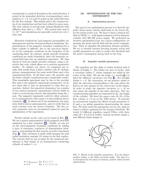
The impellers are flat disks of radius R fitted with 8
blades of height h. The blades are arcs of circles, with
a curvature radius C, whose tangents are radial at the
center of the disks. We use the angle α = arcsin( R
2C ) to
label the different curvatures (see Fig. 3). For straight
blades α = 0. By convention, we use positive values to
label the direction corresponding to the case where the
fluid is set into motion by the convex face of the blades.
In order to study the opposite curvature (α < 0) we
just rotate the impeller in the other direction. The two
counterrotating impellers are separated by H c , the height
of the cylinder. We fixed the aspect ratio H c /R c of the
flow volume to 1.8 as in the VKS device. In practice
we successively examine the effects of each parameter h,
R and α on global quantities characterizing the mean
flow. We then varied the parameters one by one, until we
found a relative optimum for the dynamo threshold. We
tested 12 different impellers, named TMxx, with three
radii (R = 0.5, 0.75 & 0.925), various curvature angles α
and different blade heights h.
+
R
α
v ≡ v measured for 0 ≤ r ≤ 1
v ≡ 0 for 1 < r ≤ 1 + w
FIG. 3: Sketch of the impeller parameters. R is the dimensionless
radius, α the blade curvature angle. The sign of α
is determined by the sense of rotation: positive when rotated
anticlockwise.