Kernel Home Range Estimation for ArcGIS, using VBA - Fish and ...
Kernel Home Range Estimation for ArcGIS, using VBA - Fish and ...
Kernel Home Range Estimation for ArcGIS, using VBA - Fish and ...

Create successful ePaper yourself
Turn your PDF publications into a flip-book with our unique Google optimized e-Paper software.
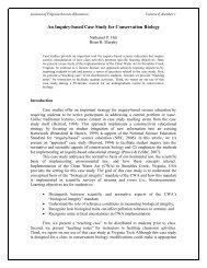
a b c<br />
Figure 6.2.1. Core area determination following Powell (2000) <strong>and</strong> Horner <strong>and</strong> Powell (1990),<br />
with r<strong>and</strong>om (a), even (b) <strong>and</strong> clumped (c) use of space (Adapted from Powell, 2000).<br />
In reality things are not this simple. R<strong>and</strong>om use of space may result in small clumps in the data<br />
(Powell, 2000). At very high probabilities of use, there may be a concave shape in the graph. In<br />
addition to this, the distribution with r<strong>and</strong>om use, will not be everywhere r<strong>and</strong>om, since the<br />
location estimates fall-off at the periphery. So, at the edges of the distribution, the probability of<br />
use will be significantly lower than everywhere else within the middle of the distribution. Thus, a<br />
core area will be indicated <strong>for</strong> every distribution that has truly ‘r<strong>and</strong>om’ or ‘even’ use, only<br />
because the probability of use increases significantly just inside the edge of the distribution.<br />
Figure 6.2.2.a., is a cross section of a kernel density estimate <strong>for</strong> r<strong>and</strong>om use, where A <strong>and</strong> B are<br />
two points at the edge of the distribution. Plotted <strong>using</strong> Powell’s (2000) method, the area<br />
contoured <strong>for</strong> a low probability of use will be large (high value on y-axis, but low value on the x-<br />
axis) while that contoured <strong>for</strong> a large probability of use will be much greater (Figure 6.2.2.b.). In<br />
Figure 6.2.2.b., the kernel density cross section is inverted <strong>and</strong> rotated so that the axes of the<br />
probability plot <strong>and</strong> that of the kernel plot will roughly match up. In theory, an even distribution<br />
should produce a graph that is flat (equal area value) <strong>for</strong> all probability of use values. There<br />
should only be one value <strong>for</strong> probability of use, since it is everywhere equal. In reality, at the<br />
edge of the distribution probability of use will be lower than the middle but will increase slightly<br />
be<strong>for</strong>e remaining constant, moving inwards from the edge (Figure 6.2.3.a.). The result of this<br />
kernel density cross section can be seen in Figure 6.2.3.b., where there will be a core estimated<br />
at a very low probability of use (near the boundary of the used area). Finally, in a clumped<br />
distribution, as with normally distributed locations (Figure 6.2.4.a.), a true concave pattern is<br />
evident in the probability plot (Figure 6.2.4.b.). Here the point where the core should be<br />
contoured is where the probability of use increases significantly (indicated by a slope m = -1).<br />
34