Chapter 5 Discrete Distributions

5.4. EXPECTATION AND MOMENT GENERATING FUNCTIONS 119
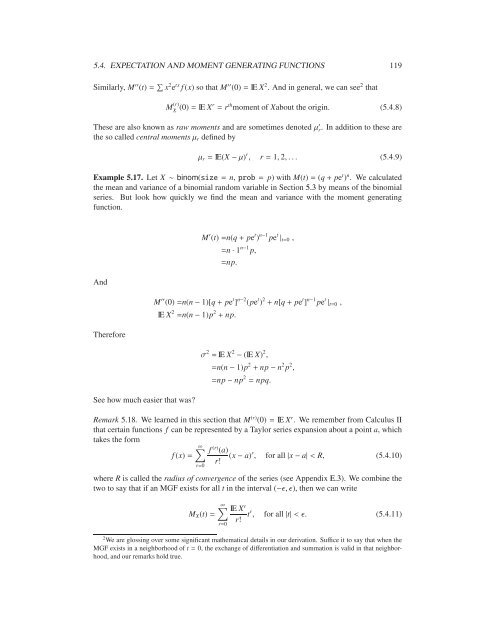
Similarly, M ′′ (t) = ∑ x 2 e tx f (x)sothatM ′′ (0) = IE X 2 .Andingeneral,wecansee 2 that
M (r)
X (0) = IE Xr = r th moment of Xabout the origin. (5.4.8)
These are also known as raw moments and are sometimes denoted µ ′ r.Inadditiontotheseare
the so called central moments µ r defined by
µ r = IE(X − µ) r , r = 1, 2,... (5.4.9)
Example 5.17. Let X ∼ binom(size = n, prob = p)withM(t) = (q + pe t ) n .Wecalculated
the mean and variance of a binomial random variable in Section 5.3 by means of the binomial
series. But look how quickly we find the mean and variance with the moment generating
function.
And
Therefore
See how much easier that was
M ′ (t) =n(q + pe t ) n−1 pe t | t=0 ,
=n · 1 n−1 p,
=np.
M ′′ (0) =n(n − 1)[q + pe t ] n−2 (pe t ) 2 + n[q + pe t ] n−1 pe t | t=0 ,
IE X 2 =n(n − 1)p 2 + np.
σ 2 = IE X 2 − (IE X) 2 ,
=n(n − 1)p 2 + np − n 2 p 2 ,
=np − np 2 = npq.
Remark 5.18. We learned in this section that M (r) (0) = IE X r .WerememberfromCalculusII
that certain functions f can be represented by a Taylor series expansion about a point a, which
takes the form
∞∑ f (r) (a)
f (x) = (x − a) r , for all |x − a| < R, (5.4.10)
r!
r=0
where R is called the radius of convergence of the series (see Appendix E.3). We combine the
two to say that if an MGF exists for all t in the interval (−ɛ, ɛ), then we can write
M X (t) =
∞∑ IE X r
t r , for all |t| < ɛ. (5.4.11)
r!
r=0
2 We are glossing over some significant mathematical details inourderivation.Suffice it to say that when the
MGF exists in a neighborhood of t = 0, the exchange of differentiation and summation is valid in that neighborhood,
and our remarks hold true.