Chapter 5 Discrete Distributions
Chapter 5 Discrete Distributions
Chapter 5 Discrete Distributions

Create successful ePaper yourself
Turn your PDF publications into a flip-book with our unique Google optimized e-Paper software.
5.6. OTHER DISCRETE DISTRIBUTIONS 127<br />
Again it is clear that f (x) ≥ 0andwecheckthat ∑ f (x) = 1(seeEquationE.3.9 in Appendix<br />
E.3):<br />
∞∑<br />
∞∑<br />
p(1 − p) x =p q x 1<br />
= p<br />
1 − q = 1.<br />
x=0<br />
We will find in the next section that the mean and variance are<br />
µ = 1 − p<br />
p<br />
x=0<br />
= q p and σ2 = q p 2 . (5.6.6)<br />
Example 5.21. The Pittsburgh Steelers place kicker, Jeff Reed, made 81.2% of his attempted<br />
field goals in his career up to 2006. Assuming that his successive field goal attempts are approximately<br />
Bernoulli trials, find the probability that Jeff misses at least 5 field goals before his<br />
first successful goal.<br />
Solution: IfX = the number of missed goals until Jeff’s first success, then X ∼ geom(prob =<br />
0.812) and we want IP(X ≥ 5) = IP(X > 4). We can find this in R with<br />
> pgeom(4, prob = 0.812, lower.tail = FALSE)<br />
[1] 0.0002348493<br />
Note 5.22. Some books use a slightly different definition of the geometric distribution. They<br />
consider Bernoulli trials and let Y count instead the number of trials until a success, so that Y<br />
has PMF<br />
f Y (y) = p(1 − p) y−1 , y = 1, 2, 3,... (5.6.7)<br />
When they say “geometric distribution”, this is what they mean. It is not hard to see that the<br />
two definitions are related. In fact, if X denotes our geometric and Y theirs, then Y = X + 1.<br />
Consequently, they have µ Y = µ X + 1andσ 2 Y = σ2 X .<br />
The Negative Binomial Distribution<br />
We may generalize the problem and consider the case where we wait for more than one success.<br />
Suppose that we conduct Bernoulli trials repeatedly, noting the respective successes and<br />
failures. Let X count the number of failures before r successes. If IP(S ) = p then X has PMF<br />
( ) r + x − 1<br />
f X (x) = p r (1 − p) x , x = 0, 1, 2,... (5.6.8)<br />
r − 1<br />
We say that X has a Negative Binomial distribution and write X ∼ nbinom(size = r, prob =<br />
p). The associated R functions are dnbinom(x, size, prob), pnbinom, qnbinom, and<br />
rnbinom, whichgivethePMF,CDF,quantilefunction,andsimulaterandom variates, respectively.<br />
As usual it should be clear that f X (x) ≥ 0andthefactthat ∑ f X (x) = 1followsfroma<br />
generalization of the geometric series by means of a Maclaurin’s series expansion:<br />
1<br />
∞∑<br />
1 − t = t k , for −1 < t < 1, and (5.6.9)<br />
k=0<br />
1<br />
∞∑ ( ) r + k − 1<br />
(1 − t) = t k , for −1 < t < 1. (5.6.10)<br />
r r − 1<br />
k=0