Introduction to Scientific Computing - Tutorial 13: Recapitulation

Introduction to Scientific Computing 

Tutorial 13: Recapitulation 

Bojana Rosic, 1. Februar 2013

Relative condition number 

Connection between the error in input and error in output: 

k(x) := ∂f 

∂x (x) x 

f (x) 

ɛ y = ∆y 

y 

= k(x)ɛ x = k(x) ∆x 

x 

This number is important as it shows how good some system is 

conditioned. If the relative error in input is ɛ x then the relative error 

in output is k(x)ɛ x . 

1. Februar 2013 Bojana Rosic Introduction to Scientific Computing Seite 2

Difference vs. Differential equations 

Difference 

x n+1 − x n = 2h 2 n 

Differential 

dx 

dt 

= 2t 

Apply Euler method 

x n+1 − x n = 2h 2 n 

Differential equations become difference when we apply numerical 

intergation! 


Homogeneous 

Difference 

x n+1 − x n = 0 

Solution form 

x n = Cρ n 

Characteristic 

Differential 

dx 

dt 

= 0 

Solution form 

x(t) = Ce ρt 

Characteristic 

ρ − 1 = 0 ρ = 0 

x n = C(1) n = C 

x = Ce 0t = C 


Homogeneous — roots 

Difference 

Differential 

Single roots ρ i 

x n = ∑ i C iρ n i 

Single roots ρ i 

x(t) = ∑ i C ie ρ it 

Double roots ρ 1 Double roots ρ 1 

x n = C 1 ρ n 1 + nC 2ρ n 1 

x(t) = C 1 e ρ 1t + tC 2 e ρ 1t 


Homogeneous — roots 

Difference 

Complex ρ = α ± βi 

Differential 

Complex ρ = α ± βi 

µ := √ α 2 + β 2 

tan φ = β/α 

x n = µ n (Acos(nφ) + iBsin(nφ)) 

x = e αt (Acos(βt) + iBsin(βt)) 


Non-homogeneous- Particular solution 

Difference 

Differential 

x n = x nh + x np 

x = x h + x p 

x h = Ce pt , x p = c(t)e pt 

variation of constant 


Stability 

Difference 

x n+1 = F(x n ) 

Differential 

dx 

dt 

= f (x) 

x ∗ = F(x ∗ ) f (x ∗ ) = 0 

[λ, v] = eig DF(x ∗ ) [λ, v] = eig Df (x ∗ ) 

(λ) n ⇒ abs (λ) 1 (real) 

e λt ⇒ abs (λ) 0 (real) 

abs (µ) 1 (complex) 

abs (α) 0 (complex) 

Remember that eigenvalues are equal to roots of charact. eq.!! 


Stability 

If there is just one root equal to 1 (i.e. 0) ⇒ stable but not asympt. 

(1) n = 1, e 0t = 1, n → ∞ & t →→ ∞ 

If there are more than one root equal to 1( i.e. 0) ⇒ not stable 

c 1 (1) n +c 2 n(1) n → ∞, c 1 e 0t +c 2 te 0t → ∞, n → ∞ & t →→ ∞ 


Zero-stability 

Test numerical method on ODE: 

for example Euler: 

write characteristic equation 

ẋ = 0 

x n+1 − x n = 0 

p − 1 = 0 ⇒ p = 1 

and find roots. Check if they are by absolute value less or equal to 

one (THIS IS DIFFERENCE EQ.). If yes then the method is 

zero-stable. 


Consistency 

Write numerical method for ODE 

in a form: 

1 

h 

ẋ = f (t, x) 

k∑ 

x n+k−i = ϕ f (t, x n+k , ..., x n , h) 

i=0 

Then find characteristic polynomial ρ(ξ) when ϕ f = 0 and its roots 

ξ. Then the method is consistent if 

and 

is equal to function f . 

ρ(1) = 0 

ϕ f (t, x, x, .., x, o) 

ρ ′ (1) 


Convergence 

Method is convergent if it is consistent and zero-stable. 


Numerical Integration of ODEs 

ẋ = f (t, x) 

Mid-point rule: 

x n+1 = x n + f (t n + h 2 , x n + h 2 f (t n, x n )) 

Trapezoidal rule: 

) 

x n+1 = x n + 1 2 

(f h (t n , x n ) + f (t n+1 , x n+1 ) 

Read also Simpson’s rule, Lagrange interpolation 

1. Februar 2013 Bojana Rosic Introduction to Scientific Computing Seite 13

Linear multi-step methods 

k∑ 

k∑ 

α j x n+j = h β j f n+j , α k = 1, |α 0 | + |β 0 | ≠ 0 

j=0 

j=0 

where f n+j = f (t n+j , x n+j ). 

Euler’s explicit method: 

x n+1 = x n + hf (t n , x n ) 

Euler’s implicit method: 

x n+1 = x n + hf (t n+1 , x n+1 ) 


Stability of linear multistep method 

Dalquist problem: 

i.e. 

k∑ 

α j x n+j = h 

j=0 

Let z := hλ and : 

ẋ = λx 

k∑ 

β j f n+j , α k = 1, |α 0 | + |β 0 | ≠ 0 

j=0 

k∑ 

α j x n+j = hλ 

j=0 

ρ(ξ) := 

k∑ 

β j x n+j 

j=0 

k∑ 

α j ξ j 

j=0 

be characteristic equation for LHS ∑ k 

j=0 α jx n+j = 0 


Stability of linear multistep method 

and 

σ(ξ) := hλ 

k∑ 

β j x j 

characteristic polynomial for RHS ∑ k 

j=0 β jf n+j = 0. Then stability is 

determined by roots 

ρ(ξ) − zσ(ξ) = 0 

i.e. region: 

G s := {z ∈ C : |ξ l | 1and if ξ l is multiple root then |ξ l | < 1} 

j=0 


Runge-Kutta methods 

The general form of explicit Runge-Kutta method is: 

where 

s∑ 

y n+1 = y n + h b i k i 

i=1 

k 1 = f (t n , y n ) 

k 2 = f (t n + c 2 h, y n + a 21 k 1 h), 

k 3 = f (t n + c 3 h, y n + (a 31 k 1 + a 32 k 2 )h), 

. 

k s = f (t n + c s h, y n + h(a s1 k 1 + a s2 k 2 + · · · + a s,s−1 k s−1 )) 

and b i are coefficients. 


Solving linear system of equations 

System: 

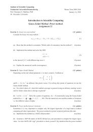
Gauss-Seidel method: 

Ax = b 

Lx (k+1) = b − Ux (k) 

Jacobi method: 

Dx (k+1) = b − Rx (k) 

Successive over-relaxation (SOR) method: 

x (k+1) = (D + ωL) −1( ωb − [ωU + (ω − 1)D]x (k)) . 


Fixed-point iterations 

We want to solve 

Φ(x) = x 

such that 

Φ has fixed point (solution) 

the fixed point is unique 

can be obtained by iterative process 

Φ is also called mapping. 


Fixed-point iterations 

Banach fixed point 

Lipshitz continuity (for q 0): 

If this holds when 0 q < 1 then 

‖Φ(x) − Φ(y)‖ q‖x − y‖ 

Φ(x ∗ ) = x ∗ has unique solution 

for any initial value sequence x n+1 = Φ(x n ) converges to 

solution x ∗ (this means that iterative method is convergent and 

gives the solution) 

speed of convergence are given by apriori and aposteriori 

estimates 


Newton method 

F(x) = 0 

F(x) = F(x 0 ) + F ′ (x 0 )(x − x 0 ) + h.o.t. = 0 

Jacobian: 

with elements: 

Newton iteration: 

J(x) = F ′ (x) 

J ij = ∂f i 

∂x j 

x k = x k−1 − F(x k−1) 

J(x k−1 ) 


Previous homework! 


Previous HW- Runge-Kutta-Fehlberg method 

Let us observe the ODE of form: 

˙u = f (t, u(t)), u(t 0 ) = u 0 

and find the Taylor expansion of solution: 

p∑ u k 

U := u m+1 = u m + 

k! hk + O(h p+1 ). 

k=1 

The 2(3)-stage Runge–Kutta–Fehlberg-method is given as 

k 1 = f (t, u) 

k 2 = f (t + c 2 h, u + ha 21 k 1 ) 

k 3 = f (t + c 3 h, u + ha 31 k 1 + ha 32 k 2 ) 

2∑ 

u m+1 = u m + h b i k i , û m+1 = u m + h 

i=1 

1. Februar 2013 Bojana Rosic Introduction to Scientific Computing Seite 23 

3∑ 

ˆb i k i . 

i=1


As k’s do not depend directly on u and t let us expand it in Taylor 

serie: 

k 1 = f 

k 2 = f + c 2 hf t + ha 21 ff u + h2 

2 [c2 2 f tt + 2c 2 a 21 ff tu + a21 2 f 2 f uu ] 

k 3 = f + c 3 hf t + h(a 31 k 1 + a 32 k 2 )f u 

+ h2 

2 [c2 3 f tt + 2c 3 (a 31 k 1 + a 32 k 2 )f tu + (a 31 k 1 + a 32 k 2 ) 2 f uu ] 

= f + h[c 3 hf t + (a 31 + a 32 )ff u ] 

+ h2 

2 [c2 3 f tt + 2c 3 (a 31 + a 32 )ff tu + (a 31 + a 32 ) 2 f 2 f uu ] 

+h 2 a 32 (c 2 f t + a 21 ff u )f u . 



Then, having that: 

2∑ 

W := u m+1 = u m + h b i k i , 

i=1 

3∑ 

Ŵ := û m+1 = u m + h ˆb i k i . 

i=1 

we may find the local truncation error: 

T h = U − W , 

ˆTh = U − Ŵ 

in which we will explit the fact a 31 + a 32 = c 3 



T h = U − W 

= hf [1 − b 1 − b 2 ] + h 2 [( 1 

2 − b 2c 2 

) 

f t + 

+O(h 3 ) 

ˆT h = U − Ŵ 

( 1 

2 − b 2a 21 

) 

ff u 

] 

( ) 

= hf [1 − ˆb 1 − ˆb 2 − ˆb 3 ] + h 2[ 1 

2 − ˆb 2 c 2 − ˆb 3 c 3 f t 

( ) [ 1 

+ 

2 − ˆb 2 a 21 − ˆb 

] 

3 c 3 ff u + h 

3 1 

6 − 1 2 ˆb 2 c2 2 − 1 ] 

2 ˆb 3 c3 

2 f tt + 



[ ] [ ] 

1 1 

+h 3 6 − c 2a 21ˆb2 − c3 

2 ff tu + h 3 6 − a2 21ˆb 2 − c3 

2 f uu 

[ ] [ ] 

1 1 

+h 3 6 − a 32c 2ˆb3 f t f u + h 3 6 − a 32a 21ˆb3 f 2 fu 2 . 

From b 2 a 21 = 1 2 and b 2c 2 = 1 2 follows a 21 = c 2 . Thus, the following 

equalities have to be fullfilled: 

b 1 + b 2 = 1 

b 2 c 2 = 1 2 

ˆb 1 + ˆb 2 + ˆb 3 = 1 

ˆb 2 c 2 + ˆb 3 c 3 = 1 2 



ˆb 2 c 2 2 + ˆb 3 c 2 3 = 1 3 

a 32 c 2ˆb3 = 1 6 . 

Let c 2 and c 3 be free parameters. Then from 

b 2 = 1 

2c 2 

and with 

b 1 = 2c 2 − 1 

2c 2 


we may find ˆb 2 and ˆb 3 as well as ˆb 1 (solve previous system): 

ˆb 1 = 6c 2c 3 + 2 − 3(c 2 + c 3 ) 

6c 2 c 3 

ˆb 2 = 

3c 3 − 2 

6c 2 (c 3 − c 2 ) 

ˆb 3 = 

2 − 3c 2 

6c 3 (c 3 − c 2 ) 

a 32 = c 3(c 3 − c 2 ) 

c 2 (2 − 3c 2 ) 


Previous HW- Skydiver mechanics 

Fall without parachute t = [0, 5]: 

m = 140 kg 

m dv 

dt 

= mg − 0.5v, v(0) = 0 

Fall with parachute t = [5, 30]: 

m dv 

dt 

= mg − 70v 2 

Initial condition in second is the last solution from first. 


Previous HW- Skydiver mechanics I way 

First five seconds: 

m dv 

dt 

= mg − 0.5v, v(0) = 0 

Algebraic solution: 

2m dv 

dt 

= 2mg − v, v(0) = 0 

dv 

2mg − v = 1 

2m dt 

∫ 

∫ 

dv 1 

2mg − v = 2m dt 




∫ 

∫ 

dv 1 

2mg − v = 2m dt 

Take p := 2mg − v then dp = −dv: 

∫ dp 

p = − ∫ 1 

2m dt 

i.e. 

v = 2mg − Ce − 1 

2m t , 

ln p = − 1 

2m t + ln C 

p = Ce − 1 

2m t 

v(0) = 0 ⇒ C = 2mg 


Previous HW- Skydiver mechanics II way 


m dv 

dt 

= mg − 0.5v, v(0) = 0 

Algebraic solution: 

dv 

dt + 1 

2m v = g 

Thus equation is inhomogeneous. Homogeneous solution comes 

from characteristics equation: 

i.e. homogeneous solution is: 

p + 1 

2m = 0 ⇒ p = − 1 

2m 

v h = C h e − 1 

2m t 



Particular solution is obtained by the method of variation of 

constant: 

v p = C p (t)e − 2m 1 t 

Putting back in original ODE: 

dv p 

dt 

= C ′ pe − 1 

2m t − 1 

2m C p(t)e − t 

2m 

dv p 

dt 

+ 1 

2m v p = g 

C ′ pe − 1 

2m t = g ⇒ C p (t) = 2mge t 

2m 

v p = 2mg 



The final solution is then: 

v = v h + v p 

v = C h e − t 

2m + 2mg 

From initial condition v(0) = 0 one obtains: 

v(0) = C h + 2mg = 0 ⇒ C h = −2mg 

v = 2mg − 2mge − t 

2m 

= 2mg(1 − e 

− t 

2m ) 



Let us now solve the second part for time interval after 5s: 

m dv 

dt 

i.e. let us divide it by m: 

then 

= mg − kv 2 , k = 70 

m 

k 

m 

k 

dv 

dt 

mg 

k 

= mg 

k 

− v2 

dv 

= dt 

− v2 

∫ 

dv 

√ = k ∫ 

dt 

( mg 

k )2 − v 2 m 



∫ 

dv 

√ = k ∫ 

dt 

( mg 

k )2 − v 2 m 

√ 

mg 

1 

k 

√ ln | √ 

2 mg mg 

k k 

√ 

mg 

k 

√ 

mg 

k 

+ v 

+ v 

− v = Ce k m 2√ mg 

v = 

√ 

mg 

k 

− v | = k m t + ln C 

k t = Ce 2 √ 

kg 

m t 

√ 

Ce 2 kg 

m t − 1 

√ 

Ce 2 kg 

m t + 1 



Initial condition is found from the solution of first ODE: 

v(5) = 2mg(1 − e − 5 

2m ) 

and substituted to: 

Euler method: 

v(5) = 

√ 

mg 

k 

√ 

Ce 2 kg 

m 5 − 1 

√ 

Ce 2 kg 

m 5 + 1 

v n+1 = v n + hf (v n , t n ) 


MATLAB 

% main script 

clear variables;clc 

v=0; 

h=0.001; 

tstart=0; 

tend=30; 

[vv,vtrue,tt,err]=jump(h,tstart,tend,v); 


MATLAB 

function [vv,vtrue,tt,err]=jump(h,tstart,tend,v) 

% jumping function :) 

n=abs(tstart−tend)/h; 

t=tstart; 

vtrue=[]; 

err=[]; 

for i=1:n 

vv(i)=v; 

tt(i)=t; 


MATLAB 

if t

MATLAB 

function v=funode1(v,t) 

v=10−0.5/140*v; 

function v=funode2(v,t) 

v=10−0.5*v*v; 

function vout=fun1(t) 

v=dsolve('Dy=10−y/(2*140)','y(0)=0'); 

vout=subs(v,t); 

function vout=fun2(t) 

v=dsolve('Dy=10−0.5*y^2','y(5)=49.55'); 

vout=subs(v,t);

Introduction to Scientific Computing - Tutorial 13: Recapitulation

Create successful ePaper yourself

Delete template?

Save as template?