Introduction to Scientific Computing - Tutorial 13: Recapitulation

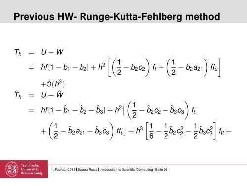
Previous HW- Runge-Kutta-Fehlberg method
T h = U − W
= hf [1 − b 1 − b 2 ] + h 2 [( 1
2 − b 2c 2
)
f t +
+O(h 3 )
ˆT h = U − Ŵ
( 1
2 − b 2a 21
)
ff u
]
( )
= hf [1 − ˆb 1 − ˆb 2 − ˆb 3 ] + h 2[ 1
2 − ˆb 2 c 2 − ˆb 3 c 3 f t
( ) [ 1
+
2 − ˆb 2 a 21 − ˆb
]
3 c 3 ff u + h
3 1
6 − 1 2 ˆb 2 c2 2 − 1 ]
2 ˆb 3 c3
2 f tt +
1. Februar 2013 Bojana Rosic Introduction to Scientific Computing Seite 26