Introduction to Scientific Computing - Tutorial 13: Recapitulation

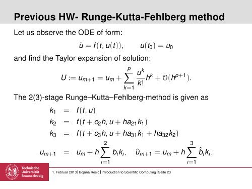
Previous HW- Runge-Kutta-Fehlberg method
Let us observe the ODE of form:
˙u = f (t, u(t)), u(t 0 ) = u 0
and find the Taylor expansion of solution:
p∑ u k
U := u m+1 = u m +
k! hk + O(h p+1 ).
k=1
The 2(3)-stage Runge–Kutta–Fehlberg-method is given as
k 1 = f (t, u)
k 2 = f (t + c 2 h, u + ha 21 k 1 )
k 3 = f (t + c 3 h, u + ha 31 k 1 + ha 32 k 2 )
2∑
u m+1 = u m + h b i k i , û m+1 = u m + h
i=1
1. Februar 2013 Bojana Rosic Introduction to Scientific Computing Seite 23
3∑
ˆb i k i .
i=1