Chapter 7: The Riemann Integral When the derivative is introduced ...

Chapter 7: The Riemann Integral
When the derivative is introduced, it is not hard to see that the limit of the difference quotient
should be equal to the slope of the tangent line, or when the horizontal axis is time and the vertical
is distance, equal to the instantaneous velocity. But the integral is not so easily interpreted: Why
is the area under the curve in any way related to the antiderivative It really was a stroke of genius
by Newton and Leibnitz to see that connection.
In fact, integration, in the sense of area or volume, was invented first, many centuries earlier:
Archimedes was involved in trying to compute the volume of a wine cask. The derivative was a
much harder concept. In fact, Zeno’s paradoxes show how hard the Greeks found the concept of
limit in general. Differentiation could really only be recognized and investigated after Descartes
invented coordinate geometry. As a result, a few calculus texts, seeking a “historical” approach to
the subject, cover integration before differentiation.
Definition. Let f be a bounded function on a compact interval [a, b]. (We’ll see later why the
underlined words are important. For now, just note that we are not assuming that f is even
continuous.)
(a) A partition P of [a, b] is a finite subset of [a, b] containing a and b. If Q is another partition
and P ⊆ Q, then Q is a refinement of P .
(b) Write P = {x 0 , x 1 , x 2 , . . . , x n } where a = x 0 < x 1 < x 2 < · · · < x n = b. Then
U(f, P ) =
L(f, P ) =
n∑
sup{f(x) : x i−1 ≤ x ≤ x i }(x i − x i−1 )
i=1
n∑
inf{f(x) : x i−1 ≤ x ≤ x i }(x i − x i−1 )
i=1
are the upper and lower sums with respect to f and P .
(c) The upper and lower integrals of f on [a, b] are U(f) = inf{U(f, P )} and L(f) = sup{L(f, P )},
where the inf and sup are taken over all partitions P of [a, b].
(d) If U(f) = L(f), then f is integrable on [a, b], and their common value is denoted ∫ b
a f or
f(x) dx.
∫ b
a
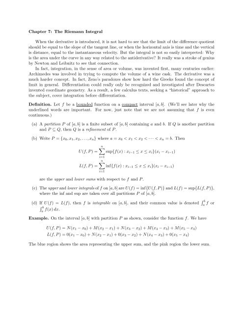
Example. On the interval [a, b] with partition P as shown, consider the function f. We have
U(f, P ) = N(x 1 − x 0 ) + M(x 2 − x 1 ) + N(x 3 − x 2 ) + M(x 4 − x 3 ) + M(x 5 − x 4 )
L(f, P ) = 0(x 1 − x 0 ) + N(x 2 − x 1 ) + 0(x 3 − x 2 ) + N(x 4 − x 3 ) + 0(x 5 − x 4 )
The blue region shows the area representing the upper sum, and the pink region the lower sum.

With a partition Q that refines P , the upper sum decreases and the lower sum increases:
Replacing the partitions with ever finer ones, we see that the upper sums and lower sums approach
each other, with the area of the three triangles as the common limit: U(f) = L(f) = ∫ b
a f.

We see now why we restricted to bounded functions: So that the sup and inf of f on each
subinterval exists (and is finite). And similarly we restricted to bounded intervals so that we do
not have infinitely long subintervals or infinitely many subintervals, making the upper and lower
sums much harder or impossible to interpret. (We restricted to closed intervals so that the function
has values at the endpoints.) Later in a calculus course integrals of unbounded functions or over
unbounded or unclosed intervals might be allowed, but such things are always called “improper
integrals” and interpreted as limits of proper integrals, limits that may or may not exist:
Example. Improper integrals:
∫ 1
0
∫ ∞
1
∫ ∞
−∞
1
√ x
dx = lim
1
√ x
dx =
ε→0 + ∫ 1
lim
M→∞
sin x dx = lim
M→∞
ε
∫ M
1
√ x
dx = lim
1
∫ M
The correct version of the last one is
−M
1
√ x
dx =
sin x dx =
[
2x 1/2] 1
ε→0 +
lim
M→∞
[2x 1/2] M
= lim 2(1 − √ ε) = 2
ε ε→0 +
1 = lim
M→∞ 2(√ M − 1) = ∞
lim [− cos
M→∞ x]M −M = lim 0 = 0
M→∞
∫ ∞
−∞
sin x dx =
lim
lim
N→−∞ M→∞
∫ M
N
sin x dx =
lim
N→−∞
lim [− cos M→∞ x]M N
does not exist
The limit where the left and right endpoint approach −∞ and ∞ at the same rate is the called the
“principal value of the improper integral.”
Example. A function that is not integrable: The Dirichlet function χ Q on [0, 1]. Every subinterval
in every partition contains rational numbers, so the supremum of the χ Q -values on the subinterval
is 1, so the upper sum for every partition is 1, so the upper integral is 1. But every subinterval in
every partition also contains irrational numbers, so the infimum of the χ Q -values on the subinterval
is 0, so the lower sum for every partition is 0, so the lower integral is 0.
Lemma. For any bounded function f on the compact interval [a, b]:
(a) For any partition P of [a, b], L(f, P ) ≤ U(f, P ).
(b) For any partitions P, Q of [a, b], if P ⊆ Q, then L(f, P ) ≤ L(f, Q) and U(f, P ) ≥ U(f, Q).
(c) For any partition P of [a, b], L(f, P ) ≤ U(f) Therefore, L(f) ≤ U(f).
Proof. (a) On any subinterval [x i−1 , x i ], inf{f(x) : x i−1 ≤ x ≤ x i } ≤ sup{f(x) : x i−1 ≤ x ≤ x i }.
(b) It is enough to assume that Q has only one more element than P , say P = {x 0 , x 1 , . . . , x n }
and Q has the additional division point x ∗ between x j−1 and x j . Then p = inf{f(x) : x j−1 ≤ x ≤

x j } is less than or equal to each of q 1 = inf{f(x) : x j−1 ≤ x ≤ x ∗ } and q 2 = inf{f(x) : x ∗ ≤ x ≤ x j }
— it is equal to at least one, but no larger than either. So the term p(x j − x j−1 ) in L(f, P ) that
corresponds to [x j−1 , x j ] is at most the sum q 1 (x ∗ − x j−1 ) + q 2 (x j − x ∗ ) of the two terms in L(f, Q)
that correspond to [x j−1 , x ∗ ] and [x ∗ , x j ] — because x j − x j−1 = (x ∗ − x j−1 ) + (x j − x ∗ ). Adding
up all the terms for all the subintervals in each partition, we see that L(f, P ) ≤ L(f, Q). Similarly,
U(f, P ) ≥ U(f, Q).
(c) Assume BWOC that there is a partition P for which L(f, P ) > U(f). Then L(f, P ) is not
a lower bound for the set of all upper sums, so there is a partition Q for which L(f, P ) > U(f, Q).
But then P ∪ Q is a refinement of both P and Q, so by (b) and (a), we have
L(f, P ) ≤ L(f, P ∪ Q) ≤ U(f, P ∪ Q) ≤ U(f, Q) ,
a contradiction. Thus, U(f) is an upper bound on the set of all lower sums, it is at least as large
as the least upper bound, and we have the “Therefore” sentence.
Here is another way to say “integrable”, in which, instead of finding one partition P that makes
L(f, P ) almost as large as possible and another, Q, that makes U(f, P ) almost as small as possible,
we say that it is enough to find a single partition that makes the upper and lower sums close to
each other:
Proposition. A bounded function f : [a, b] → R is integrable iff, ∀ ε > 0, ∃ P partition of [a, b] s.t.
U(f, P ) − L(f, P ) < ε.
Proof. (⇐) Assume BWOC that U(f) ≠ L(f). Then then U(f) − L(f) = ε > 0. By hypothesis,
∃ P s.t. U(f, P ) − L(f, P ) < ε. But because L(f, P ) ≤ L(f) and U(f, P ) ≥ U(f), we have
U(f) − L(f) ≤ U(f, P ) − L(f, P ) < ε = U(f) − L(f), −/\−.
(⇒) Let ε > 0 be given, and pick P, Q s.t. U(f, P ) − ∫ b
a f < ε/2 and ∫ b
a
f − L(f, Q) < ε/2 Then
because P ∪ Q is a common refinement of P, Q, we have
so
L(f, Q) ≤ L(f, P ∪ Q) ≤ U(f, P ∪ Q) ≤ U(f, P ) ,
U(f, P ∪ Q) − L(f, P ∪ Q) ≤ U(f, P ) − L(f, Q)
( ∫ b
)
= U(f, P ) − f +
a
(∫ b
a
)
f − L(f, Q) < ε .
Now we show that a continuous function (on a compact interval) is integrable. Because not all
continuous functions are differentiable, we see that it is harder for a function to be differentiable
than for it to be integrable.
Theorem. If f : [a, b] → R is continuous, then it is integrable.
Proof. Let ε > 0 be given. Because f is uniformly continuous, there is a δ > 0 for which |x i −x j | < δ
implies |f(x i ) − f(x j )| < ε/(b − a). Pick a partition P for which all the subintervals [x i−1 , x i ] have
length less than δ. (For example, we might choose n in N so large that (b − a)/n < δ and set
P = {x i = a+i(b−a)/n : i = 0, 1, . . . , n}.) Then because f attains its inf and sup on each [x i−1 , x i ],
say at t i and u i respectively, we have |t i − u i | ≤ |x i − x i−1 | < δ, so |f(t i ) − f(u i )| < ε/(b − a), so
U(f, P ) − L(f, P ) =
n∑
(f(t i ) − f(u i ))(x i − x i−1 ) <
i=1
n∑
i=1
ε
b − a (x i − x i−1 ) =
ε
b − a (x n − x 0 ) = ε ,

the second last equality because the sum
(x 1 − x 0 ) + (x 2 − x 1 ) + · · · + (x n − x n−1 )
“telescopes”, i.e., all the terms cancel except the second and second last.
But there are many discontinuous integrable functions; our first example (the “three triangles”)
was discontinuous at two points but still integrable. We have seen that the Dirichlet function on
[0, 1] is not integrable. But we claim that the Thomae function is integrable on this interval:
Example. Recall that the Thomae function is given by
{ 0 if x is irrational
t(x) = 1
n
if x = m n
in lowest terms
Because every subinterval of every partition of [0, 1] contains irrational numbers, the lower sum of t
with respect to every partition is 0, so the lower integral of t is 0. Thus, to see that t is integrable,
we need to show that the upper integral is 0, i.e., that, given ε > 0, we can find a partition P with
respect to which U(t, P ) < ε. We can do that: There are only finitely many rationals x in [0, 1] for
which f(x) > ε/2. Pick a partition P of [0, 1] so that these finitely many rationals are the centers
(or, for x = 0 and x = 1, the ends) of subintervals with total length ε/2. Then in U(f, P ), the terms
corresponding to those subintervals add up to at most 1 times the total length of these subintervals
and hence less than ε/2. In the other subintervals the value of the function is at most ε/2, so those
subintervals contribute to U(f, P ) a total of less than (ε/2) · 1. It follows that U(f, P ) < ε.
In fact, it is shown in the text that a bounded function on a compact interval is integrable iff its
set of discontinuities has “measure zero.” We won’t try to explain this term, because the right way
to do that is to take a totally different approach to the course, in terms of “Lebesgue integration.”
So we will only say that all countable sets, including finite sets, and the Cantor set have “measure
zero,” so that functions that are discontinuous only on these sets are integrable. (“Measure” is
a concept that extends the idea of length, so a set of length l has measure l; but it is hard to
assign a “length” to a set like the rationals, which has measure 0.) Remember that the Dirichlet
function is discontinuous everywhere, so its set of discontinuities in [0, 1] has measure one; but the
Thomae function is discontinuous only on the rationals, which have measure 0. And sure enough,
the Dirichlet function is not integrable, while the Thomae function is.
[At this point students are ready to do the eleventh problem set.]
Proposition. (Properties of the definite integral) Suppose f, g are integrable on [a, b] and k
is a constant. Then:
(0) If a < c < b, then ∫ b
a f = ∫ c
a f + ∫ b
c f.
(1) ∫ b
a (f + g) = ∫ b
a f + ∫ b
a g.
(2) ∫ b
a kf = k ∫ b
a f.
(3) If f ≤ g on [a, b], then ∫ b
a f ≤ ∫ b
a g.
Corollary. (of (3)): (3a) If m ≤ f ≤ M on [a, b], then m(b − a) ≤ ∫ b
a
f ≤ M(b − a).
(3b) |f| is integrable and | ∫ b
a f| ≤ ∫ b
a |f|.

The fact that |f| is integrable is new information — the proof is an exercise. To do it, you
should verify that, if m i , M i are the inf and sup of f on [x i−1 , x i ] and m ′ i , M i ′ are the same for |f|,
then M i − m i ≥ M i ′ − m′ i . To get the second assertion in (3b), use −|f| ≤ f ≤ |f| on [a.b].
Remarks on the proposition:
(0) Part of what is to be proved here is that f is integrable on [a, b] iff it is integrable on both
[a, c] and [c, b]. But if we define ∫ a
a f = 0 and ∫ a
b f = − ∫ b
a
f, then we don’t need to add the
“If” part of this statement as long as f is integrable on the intervals determined by a, b, c.
(1) The proof is an exercise.
(2) Here is a proof of the k < 0 case: Let ε > 0 be given, and pick a partition P of [a, b] for which
U(f, P ) − ∫ b
a f < ε/(2|k|) and ∫ b
a
f − L(f, P ) < ε/(2|k|). Then because, on each subinterval
[x i−1 , x i ] in P we have
sup{kf(x) : x i−1 ≤ x ≤ x i } = k · inf{f(x) : x i−1 ≤ x ≤ x i }
and similarly with sup and inf reversed, it follows that
U(kf, P ) − L(kf, P ) = kL(f, P ) − kU(f, P ) = |k|(U(f, P ) − L(f, P ))
( ∫ b ∫ b
)
≤ |k| U(f, P ) − f + f − L(f, P ) ) < ε 2 + ε 2 = ε ,
so kf is integrable, and
U(kf, P ) − k
so k ∫ b
a f = ∫ b
a kf.//
∫ b
a
(
f = k L(f, P ) −
∫ b
a
a
a
) (∫ b
)
f = |k| f − L(f, P ) < ε
a
2 < ε ,
(3) Because f ≤ g, for any subinterval [x i−1 , x i ] of any partition P of [a, b] we have
sup{f(x) : x i−1 ≤ x ≤ x i } ≤ sup{g(x) : x i−1 ≤ x ≤ x i }
so U(f, P ) ≤ U(g, P ), so ∫ b
a f = inf P U(f, P ) ≤ inf P U(g, P ) = ∫ b
a g.
[At this point students are ready to do the twelfth problem set.]
Theorem. (Fundamental Theorem of Calculus) (1) If f is the derivative of F on [a, b] and
f is integrable, then ∫ b
a
f = F (b) − F (a).
(2) Let g : [a, b] → R be integrable, and define G(t) = ∫ t
a
g(x) dx. Then G : [a, b] → R is
continuous. If g is continuous at c in [a, b], then G is differentiable at c and G ′ (c) = g(c).
Proof. (1) For any subinterval [x i−1 , x i ] in any partition P of [a, b], by the Mean Value Theorem
∃ x ∗ i ∈ [x i−1 , x i ] s.t. F (x i ) − F (x i−1 ) = f(x ∗ i )(x i − x i−1 ), so ∑ n
i=1 (F (x i) − F (x i−1 )) is between
L(f, P ) and U(f, P ). But the sum is telescoping, to F (b) − F (a), independent of the partition P ,
so F (b) − F (a) is between L(f) and U(f), which are both equal to ∫ b
a f.

(2) In fact, we can show that G is Lipschitz, which is stronger than continuous: Let M be an
upper bound on |g| in [a, b]. Then for all x 1 , x 2 ∈ [a, b], we have
∫ x1
∫ x2
∣∫ ∣∣∣ x1
|G(x 1 ) − G(x 2 )| =
∣ g − g
∣ = g
∣ ≤ M|x 1 − x 2 | .
a
Now suppose g is continuous at c. Then
a
x 2
G ′ G(x) − G(c)
(c) = lim
= lim
x→c x − c
∫ x
c g
x→c
x − c ,
so we want to show, given ε > 0, ∃ δ > 0 s.t. 0 < |x − c| < δ =⇒ | ∫ x
c
g/(x − c) − g(c)| < ε. Now
there is a δ > 0 s.t., if |x − c| < δ, then |g(x) − g(c)| < ε, and for that δ, if 0 < |x − c| < δ, then
∫ x
c g ∣ (∫ ∣∣∣
∣x − c − g(c) =
1 x
∣∣∣
∣ (g(t) − g(c))dt)∣
x − c c
≤ 1 ∫ x
|g(t) − g(c)|dt ≤ 1 ∫ x
ε dt = ε .
x − c
x − c
(In the middle of this, note that, if x−c < 0, then any ∫ x
c
∫ x
c
c
c
of a nonnegative function is also ≤ 0.)
Here are some examples of functions g and the functions G defined by their integrals, G(x) =
g(t) dt.
Example. In these two examples, c = −2, so that, no matter what g is, G(−2) = ∫ −2
−2 g = 0.
We are interested especially in the points at which the definitions of g change from one formula to
another. First:
{ −1 if x < 0
g(x) =
,
1 if x ≥ 0
∫ x
{ ∫ x
G(x) = g(t) dt =
−2
−1 dt = −x − 2 if x < 0
−2
G(0) + ∫ x
0
1 dt = −2 + x if x ≥ 0
Here, G is differentiable except at the discontinuity x = 0 of g. Second:
{
−1 if x ≤ 1
g(x) =
,
2x − 3 if x > 1
∫ x
{ −x − 2 if x ≤ 1
G(x) = g(t) dt =
−2
G(1) + ∫ x
1 (2t − 3)dt = −3 + (x2 − 3x) − (−2) = x 2 − 3x − 1 if x > 1
Because this g is continuous at the point where its definition changes, the corresponding G is
differentiable there.
Here are the corresponding graphs, with the g’s in green and the G’s in red:

Though our text doesn’t seem to include them, I have seen in other texts examples of functions
defined by integrals where the upper, and maybe also the lower, limit(s) of integration are themselves
functions. In order to find their derivatives, we only need to throw in the Chain Rule: Suppose we
are given H(x) = ∫ f(x)
c
g(t) dt. We can isolate an intervening function: G(u) = ∫ u
c
g(t) dt. Then
H(x) = G(f(x)), so (d/dx)(H(x)) = G ′ (f(x)) · f ′ (x) = g(f(x))f ′ (x).
Example.
d
dx
∫ 5x 2 +3
2x
( ∫
exp(−t 2 ) dt = d 5x 2 +3
exp(−t 2 ) dt −
dx 0
∫ 2x
0
exp(−t 2 ) dt
= exp(−(5x 2 + 3) 2 ) · (10x) − exp(−(2x) 2 ) · 2
= 10x exp(−(5x 2 + 3) 2 ) − 2 exp(−(2x) 2 ) .
)
Here, the intervening function is G(u) = ∫ u
0 exp(−t2 ) dt, so that G ′ (u) = exp(−u 2 ). There is
nothing special about 0; because exp(−t 2 ) is continuous everywhere, any constant would have
worked.
[At this point students are ready to do the thirteenth problem set.]