Modeling of Biogas Reactors
Modeling of Biogas Reactors
Modeling of Biogas Reactors

Create successful ePaper yourself
Turn your PDF publications into a flip-book with our unique Google optimized e-Paper software.
6<br />
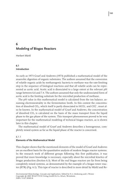
<strong>Modeling</strong> <strong>of</strong> <strong>Biogas</strong> <strong>Reactors</strong><br />
Herbert Märkl<br />
6.1<br />
Introduction<br />
As early as 1973 Graef and Andrews (1973) published a mathematical model <strong>of</strong> the<br />
anaerobic digestion <strong>of</strong> organic substrates. The authors assumed that the conversion<br />
<strong>of</strong> volatile organic acids by methanogenic bacteria to methane was the rate-limiting<br />
step in the sequence <strong>of</strong> biological reactions and that all volatile acids can be represented<br />
as acetic acid. Acetic acid is dissociated to a large extent at the relevant pH<br />
range between 6.6 and 7.4. The authors assumed that only the undissociated form <strong>of</strong><br />
acetic acid is the limiting substrate for the microbial production <strong>of</strong> methane.<br />
The pH value in this mathematical model is calculated from the ion balance, assuming<br />
electroneutrality in the fermentation broth. In this context the concentration<br />
<strong>of</strong> dissolved CO 2, which itself is partly dissociated to HCO 3 – and CO3 2– , must also<br />
be known. In the mathematical model <strong>of</strong> Graef and Andrews, the concentration<br />
<strong>of</strong> dissolved CO 2 is calculated on the basis <strong>of</strong> the mass transport from the liquid<br />
phase to the gas phase <strong>of</strong> the system. This transport phenomenon proved to be very<br />
important for the mathematical modeling <strong>of</strong> technical biogas reactors, as is shown<br />
later in this chapter.<br />
The mathematical model <strong>of</strong> Graef and Andrews describes a homogenous, completely<br />
mixed system as far as the liquid phase <strong>of</strong> the reactor is concerned.<br />
6.1.1<br />
Elements <strong>of</strong> the Mathematical Model<br />
This chapter shows that the mentioned elements <strong>of</strong> the model <strong>of</strong> Graef and Andrews<br />
are an excellent basis for the quantitative analysis <strong>of</strong> modern biogas reactor systems.<br />
In the research work <strong>of</strong> different groups following this first publication, it was<br />
proved that more knowledge is necessary, especially about the microbial kinetics <strong>of</strong><br />
biogas production (Section 6.3). Most <strong>of</strong> the real biogas reactors are far from being<br />
completely mixed systems, as demonstrated by the example <strong>of</strong> a biogas tower reactor<br />
(BTR) (Fig. 6.1). This type <strong>of</strong> reactor is described in more detail by Märkl and Re-<br />
Environmental Biotechnology. Concepts and Applications. Edited by H.-J. Jördening and J. Winter<br />
Copyright © 2005 WILEY-VCH Verlag GmbH & Co. KGaA, Weinheim<br />
ISBN: 3-527-30585-8<br />
163
164 6 <strong>Modeling</strong> <strong>of</strong> <strong>Biogas</strong> <strong>Reactors</strong><br />
Fig. 6.1 Elements <strong>of</strong> a mathematical model for a biogas tower reactor (BTR).<br />
inhold (1994). The typical features <strong>of</strong> the BTR are its tower shape, the modular structure,<br />
and the internal installations. Gas collecting devices are used to withdraw the<br />
fermentation gas from different levels <strong>of</strong> the reactor. These gas collectors separate<br />
the reactor into modules along the height. By means <strong>of</strong> these devices, which are<br />
equipped with valves, the gas loading and the mixing intensity can be controlled separately<br />
in each module. To avoid flotation <strong>of</strong> active biomass due to excessive gas load,<br />
an effective biomass accumulation is generated within the reactor.<br />
The biomass is represented in this reactor by free suspended microorganisms<br />
which are associated in the form <strong>of</strong> sedimentable more-or-less loose pellets (flocs).<br />
One very important point, when modeling such a reactor, is to describe the local distribution<br />
<strong>of</strong> active biomass within the reactor (Section 6.4.2).<br />
In a mathematical model the mixing behavior <strong>of</strong> the liquid phase is <strong>of</strong> similar importance<br />
(Section 6.4.1). The mixing <strong>of</strong> the BTR is caused by internal airlift loop<br />
units. Since the reactor is designed in the shape <strong>of</strong> a tower and is only fed at the bot-
tom (Fig. 6.1), the question <strong>of</strong> mixing and supplying the microorganisms in each<br />
part <strong>of</strong> the reactor with nutrients is very important during the scale-up <strong>of</strong> such a<br />
system. Besides, hydraulic mixing is important to prevent toxic concentrations <strong>of</strong><br />
substrate near the inlet <strong>of</strong> the reactor.<br />
As pointed out by Graef and Andrews (1973), the mass transport <strong>of</strong> product gas<br />
from the liquid phase to the gas phase is an essential element <strong>of</strong> the mathematical<br />
model. Local transport data as a function <strong>of</strong> the hydrodynamics for the example <strong>of</strong><br />
the biogas tower reactor is given for CO 2 and H 2S in Section 6.5 <strong>of</strong> this chapter. The<br />
last element <strong>of</strong> a mathematical model which is <strong>of</strong> high importance, especially when<br />
discussing tall reactors, is represented by the influence <strong>of</strong> the local hydrostatic pressure<br />
on the kinetics <strong>of</strong> biogas generation (Section 6.6).<br />
6.1.2<br />
Scale-Up Strategy<br />
6.1 Introduction<br />
Parameters <strong>of</strong> the mathematical model elements must be identified by experiments,<br />
and the models have to be evaluated with respect to their suitability for the design <strong>of</strong><br />
technical scale biogas reactors. The scale-up strategy is demonstrated in Figure 6.2<br />
with explanations in Table 6.1. Basic experiments are done in the laboratory. The hydrodynamic<br />
behavior and the sedimentation <strong>of</strong> non-active biomass were studied<br />
first in a small reactor unit with a height <strong>of</strong> 6.5 m. This laboratory reactor has a diameter<br />
<strong>of</strong> 0.4 m and consists <strong>of</strong> only two modules. To understand the influence <strong>of</strong><br />
Fig. 6.2 Strategy for scale-up <strong>of</strong> the biogas tower reactor, specification <strong>of</strong> reactors according to<br />
Table 6.1.<br />
165
166 6 <strong>Modeling</strong> <strong>of</strong> <strong>Biogas</strong> <strong>Reactors</strong><br />
Table 6.1 Specification <strong>of</strong> biogas reactors used for the experiments.<br />
Experiments Kinetics Hydro- Local Mass Influence <strong>of</strong><br />
dynamic Distribution Transport Hydrostatic<br />
and <strong>of</strong> Biomass <strong>of</strong> Product Pressure<br />
Liquid Gas<br />
<strong>Reactors</strong> Mixing<br />
Labor- Stirred tank reactor, active<br />
atory volume 16 L � � �<br />
Two UASB reactors with<br />
biogas recirculation, active<br />
volume 36.5 L and 39.5 L, height<br />
1.7 m and 1.95 m, respectively � �<br />
Laboratory tower reactor,<br />
height 6.5 m, diameter 0.4 m,<br />
two modules � �<br />
Pilot Pilot scale tower reactor,<br />
height 20 m, diameter 1 m,<br />
volume 15 m 3 , four modules,<br />
photo <strong>of</strong> reactor shown in Figure 6.3 � � � � �<br />
Fig. 6.3 <strong>Biogas</strong> tower reactor, pilot<br />
scale, at the site <strong>of</strong> Deutsche Hefewerke<br />
in Hamburg, built by Preussag<br />
Wassertechnik GmbH, Bremen.
Table 6.2 Characteristic data <strong>of</strong> the wastewater used for the experiments.<br />
the height <strong>of</strong> a reactor, a pilot scale biogas reactor was built at the site <strong>of</strong> a company<br />
producing bakers’ yeast (Fig. 6.3). The reactor was designed on the basis <strong>of</strong> the laboratory<br />
scale experiments and investigations on the kinetics <strong>of</strong> wastewater digestion<br />
from bakers’ yeast production. The characteristic data <strong>of</strong> the wastewater are given in<br />
Table 6.2. The active volume <strong>of</strong> the reactor is 15 m 3 . It is divided into four modules<br />
and at the top <strong>of</strong> the reactor a settling zone is integrated to maintain a high sludge<br />
concentration. The pilot reactor is well equipped with instruments for measuring<br />
concentrations and velocities along the height <strong>of</strong> the reactor. Because the pilot scale<br />
reactor reaches almost the height <strong>of</strong> a technical reactor (in Fig. 6.2 two reactor units<br />
with a height <strong>of</strong> 25 m and a diameter <strong>of</strong> 3.5 m are shown as examples) it is assumed<br />
that the mathematical model, which is evaluated on the pilot scale with respect to hydraulics<br />
and takes into account the influence <strong>of</strong> hydrostatic pressure, will permit<br />
prediction <strong>of</strong> the behavior <strong>of</strong> a technical scale reactor.<br />
6.2<br />
Measuring Techniques<br />
To understand the microbial degradation process and the system behavior <strong>of</strong> a biogas<br />
reactor and to establish reliable mathematical models, measuring techniques<br />
must be available – if possible – to analyze online special substances in the fermentation<br />
broth. Therefore, some new measuring techniques have been developed during<br />
the last years.<br />
6.2.1<br />
Online Measurement Using a Mass Spectrometer<br />
Average Range Unit<br />
6.2 Measuring Techniques<br />
Total organic carbon (TOC) 13.8 11–19 g L –1<br />
Chemical oxygen demand (COD) 31 25–36 g L –1<br />
COD (incl. betaine) 44 g L –1<br />
Betaine 5.7 4–10 g L –1<br />
Sulfate 3.9 2.5–6.5 g L –1<br />
Acetic acid 58 0.6–120 mmol L –1<br />
Total suspended solids (TSS) 2.5 0.8–3 g L –1<br />
pH 4.5 4.3–5 –<br />
The anaerobic treatment <strong>of</strong> wastewater loaded with high concentrations <strong>of</strong> sulfate is<br />
<strong>of</strong>ten accompanied by problems due to inhibition by hydrogen sulfide (H 2S). It is<br />
well established that the inhibition is caused by undissociated hydrogen sulfide<br />
present in the liquid phase and not by the total sulfide content. This concentration<br />
<strong>of</strong> undissociated hydrogen sulfide depends on sulfate concentration in the wastewa-<br />
167
168 6 <strong>Modeling</strong> <strong>of</strong> <strong>Biogas</strong> <strong>Reactors</strong><br />
ter, pH, and ionic strength. The concentration <strong>of</strong> undissociated hydrogen sulfide in<br />
the liquid phase undergoes great changes in the pH range used for anaerobic digestion,<br />
which is between 6.6 and 7.4. Since the actual concentration <strong>of</strong> dissolved H 2S<br />
cannot be calculated on the basis <strong>of</strong> the H 2S partial pressure in the biogas, because<br />
gas phase and liquid phase are not in equilibrium as is demonstrated in Section 6.5,<br />
this concentration has to be measured.<br />
Measurement on the basis <strong>of</strong> ion-sensitive electrodes proved to be very problematic,<br />
especially with respect to their stability for a long period <strong>of</strong> time. Meyer-Jens et al.<br />
(1995) developed a new type <strong>of</strong> probe connected to a mass spectrometer. The probe<br />
consists <strong>of</strong> a small tube (outer diameter 0.9 mm, inner diameter 0.7 mm) <strong>of</strong> polydimethylsilicon.<br />
The tube can be inserted directly into the fermentation liquid <strong>of</strong> the<br />
biogas reactor. The H 2S dissolved in the liquid phase penetrates the membrane and<br />
is transported by a carrier gas (technical nitrogen) to the mass spectrometer.<br />
A very simple silicon membrane probe is shown in Figure 6.4. The silicon membrane<br />
tube is arranged in a short bypass loop outside <strong>of</strong> the reactor. The fermentation<br />
liquid flows outside <strong>of</strong> the tube while the carrier gas passes inside. In Figure 6.5<br />
calibration <strong>of</strong> the measurement system is demonstrated. The calibration curve is<br />
perfectly linear within the relevant H 2S concentrations. The different gradient for<br />
Fig. 6.4 Configuration <strong>of</strong> a silicon membrane<br />
probe operated in a short bypass at the reactor<br />
(after Polomski, 1998).
desalinated water and wastewater indicates the difference in the solubility (Henry<br />
coefficient) <strong>of</strong> H 2S in desalinated water (78.2 mmol L –1 bar –1 ) and wastewater<br />
(68.5 mmol L –1 bar –1 ) at 37°C (data given by Polomski, 1998).<br />
The measurement system can also serve well for the detection <strong>of</strong> dissolved CO 2 in<br />
the biogas reactor. Figure 6.6 shows the calibration curve for CO 2 in a sample <strong>of</strong> desalinated<br />
water. Also with CO 2 the solubility (Henry coefficient) for wastewater<br />
(2.21·10 –4 mmol L –1 Pa –1 ) is 12% smaller than the literature data given for desalinated<br />
water (2.52·10 –4 mmol L –1 Pa –1 ). Matz and Lennemann (1996) used a similar<br />
silicon membrane probe for online monitoring <strong>of</strong> biotechnological processes by gas<br />
chromatographic mass spectrometric analysis. The sensitivity <strong>of</strong> the probe system<br />
could be improved considerably by an instantaneous heating <strong>of</strong> the membrane to a<br />
temperature <strong>of</strong> 200 °C. This quasi online measuring procedure had a sampling period<br />
<strong>of</strong> 15 min between two successive measuring cycles. Substances like dimethylsulfide,<br />
butanethiol, cresol, phenol, ethylphenol, and indole at concentrations<br />
between 10 and 200 ppm were detected.<br />
6.2.2<br />
Online Monitoring <strong>of</strong> Organic Substances<br />
with High-Pressure Liquid Chromatography (HPLC)<br />
6.2 Measuring Techniques<br />
Fig. 6.5 Calibration <strong>of</strong> the silicon membrane probe coupled with a mass spectrometer measuring<br />
the concentration <strong>of</strong> dissolved H 2S in desalinated water (DS water) and in the wastewater <strong>of</strong><br />
bakers’ yeast production. The ordinate gives the value <strong>of</strong> the signal with reference to the N 2 signal<br />
<strong>of</strong> the carrier gas. The abscissa is the partial pressure <strong>of</strong> H 2S, with which the liquid is in equilibrium<br />
(after Polomski 1998).<br />
Zumbusch et al. (1994) reported the simultaneous online determination <strong>of</strong> betaine<br />
(trimethylglycine), N,N-dimethylglycine (N,N-DMG), acetic and propionic acid during<br />
the anaerobic fermentation <strong>of</strong> wastewater from bakers’ yeast production. Ammonia<br />
and chloride could also be measured. The determinations were carried out by<br />
169
170 6 <strong>Modeling</strong> <strong>of</strong> <strong>Biogas</strong> <strong>Reactors</strong><br />
Fig. 6.6 Calibration <strong>of</strong> the silicon membrane probe coupled to mass spectrometer measuring<br />
the dissolved CO 2 in desalinated water (after Polomski, 1998).<br />
means <strong>of</strong> isocratic cation exchange chromatography. For the detection <strong>of</strong> betaine<br />
and N,N-DMG an ultraviolet detector was used. All other substances were detected<br />
by conductivity.<br />
Besides other organic components, such as acetic and propionic acid, betaine is<br />
the dominant organic substance in the wastewater. Up to 33% <strong>of</strong> the TOC is represented<br />
by betaine. The use <strong>of</strong> HPLC analysis combined with an automated ultrafiltration<br />
setup for online process monitoring gives interesting information about the<br />
dynamic behavior <strong>of</strong> the anaerobic process, as demonstrated in Figure 6.7. The<br />
graphs show the effect <strong>of</strong> hydrogen sulfide elimination from the fermentation broth.<br />
The concentration <strong>of</strong> undissociated H 2S was decreased by a factor <strong>of</strong> 2 (from 300 to<br />
150 mg L –1 ). During the same time biogas production increased. The concentration<br />
<strong>of</strong> acetic acid decreased while the other acids measured remained more or less<br />
stable. Betaine was completely degraded only at lower H 2S concentrations. Interestingly,<br />
the concentration <strong>of</strong> N,N-DMG, which is a metabolic product <strong>of</strong> the anaerobic<br />
degradation <strong>of</strong> betaine, is also decreased.<br />
6.3<br />
Kinetics<br />
The anaerobic degradation <strong>of</strong> organic substances is performed in a sequence <strong>of</strong><br />
biological reactions in a synthrophic cooperation <strong>of</strong> different microorganisms
6.3 Kinetics<br />
Fig. 6.7 Combined measurement with the silicon membrane probe mass spectrometer and<br />
online high-pressure liquid chromatography in a laboratory upflow anaerobic sludge blanket<br />
(UASB) reactor with and without elimination <strong>of</strong> H 2S in an external biogas recirculation loop over<br />
a period <strong>of</strong> some hundred hours (after Polomski, 1998). Online measurements were carried out<br />
in cooperation with Zumbusch et al. (1994). H 2S concentrations were detected by the silicon<br />
membrane probe and mass spectrometer.<br />
(Fig. 6.8). In a first step, complex biopolymers (lipids, proteins, carbohydrates) are<br />
split into the monomers which can be assimilated by the microbial cell. This first<br />
breakdown is catalyzed by extracellular enzymes. In a second step, fermentative bac-<br />
171
172 6 <strong>Modeling</strong> <strong>of</strong> <strong>Biogas</strong> <strong>Reactors</strong><br />
Fig. 6.8 Pathway <strong>of</strong> anaerobic biodegradation.<br />
teria form hydrogen, carbon dioxide, acetic acid, propionic acid, and further intermediary<br />
products, predominantly volatile fatty acids.<br />
Acetic acid, carbon dioxide, and hydrogen can be directly converted to methane<br />
and carbon dioxide (biogas) by methanogenic bacteria. Propionic acid as well as the<br />
other intermediates cannot be directly transformed to biogas. In an intermediate<br />
step, the so-called acetogenic bacteria have to generate acetic acid, carbon dioxide,<br />
and hydrogen which then can be converted to biogas again. Thauer et al. (1977)<br />
showed that for thermodynamic reasons the degradation <strong>of</strong> propionic acid is only<br />
possible at very low concentrations <strong>of</strong> hydrogen (1 Pa). From this argument it is<br />
clear that the acetogenic reaction which generates hydrogen can be performed only<br />
by a direct and close synthrophic cooperation with methanogenic bacteria which<br />
consume hydrogen. Sulfate, a frequent component in almost all food industries’<br />
wastewater, is almost totally converted to hydrogen sulfide.<br />
The dynamic behavior <strong>of</strong> the system is mainly controlled by the conversion <strong>of</strong> acetic<br />
acid to methane and carbon dioxide. This reaction is rather slow and, therefore, it<br />
is the bottleneck <strong>of</strong> the anaerobic digestion, as demonstrated by experiments like<br />
those shown in Figure 6.9. Whey which contains about 5% lactose, is continuously<br />
digested to biogas. At the beginning <strong>of</strong> the experiment the concentration <strong>of</strong> the different<br />
volatile acids denoted in Figure 6.9 represent a steady state. In this situation<br />
the reactor was heavily overloaded during the next 2.5 h. As a result, the concentration<br />
<strong>of</strong> acetic acid increased by a factor <strong>of</strong> 5. The concentrations <strong>of</strong> the other acids remained<br />
more or less constant. This finding supports the idea <strong>of</strong> Graef and Andrews<br />
(1973) that the conversion <strong>of</strong> acetic acid to methane and CO 2 is the rate-limiting step<br />
and that a mathematical model <strong>of</strong> the anaerobic degradation process can be reduced<br />
to this dominating reaction.<br />
This simple idea is expressed in Figure 6.10 and Eqs. 1 and 2, which describe the<br />
concentration <strong>of</strong> microorganisms x and the concentration <strong>of</strong> acetic acid Ac as a function<br />
<strong>of</strong> time.
dx<br />
dt<br />
dc Ac<br />
dt<br />
= µ (c Ac, c i) x – x (1)<br />
V · feed<br />
Vreactor V · feed<br />
Vreactor 6.3 Kinetics<br />
Fig. 6.9 Concentration <strong>of</strong> the different<br />
volatile acids as a function <strong>of</strong> the time<br />
during the continuous anaerobic degradation<br />
<strong>of</strong> whey, a byproduct <strong>of</strong> cheese<br />
production (after Märkl et al., 1983).<br />
The experiments were performed in a<br />
20 L stirred tank reactor. The graph<br />
shows the dynamic behavior <strong>of</strong> the<br />
system after being heavily overloaded<br />
with whey during the first 2.5 h <strong>of</strong> the<br />
experiment.<br />
Fig. 6.10 Mathematical model <strong>of</strong> anaerobic<br />
digestion in a stirred tank reactor.<br />
The reactor is directly fed by acetic<br />
acid (concentration in the inlet: c Ac,e).<br />
The concentration <strong>of</strong> acetic acid in the<br />
reactor is c Ac, x denotes the concentration<br />
<strong>of</strong> biomass.<br />
1<br />
= (cAc,e – cAc) – µ (cAc, ci)x (2)<br />
Y-<br />
The reactor is directly fed by acetic acid c Ac,e. The growth rate <strong>of</strong> the microorganisms<br />
is denoted as µ (c Ac, c i), and the biogas production can be assumed to be directly<br />
proportional to µ. At a first glance, this model looks very simple. The real problem<br />
when solving the equation is that we need information on the kinetics <strong>of</strong> the reaction.<br />
The growth rate µ is a function <strong>of</strong> the acetic acid concentration c Ac but may also<br />
depend on the concentrations <strong>of</strong> other substances c i. Before going into detail <strong>of</strong><br />
173
174 6 <strong>Modeling</strong> <strong>of</strong> <strong>Biogas</strong> <strong>Reactors</strong><br />
formulating this kinetic equation one should understand more about the physicochemical<br />
state <strong>of</strong> the fermentation broth.<br />
Acetic acid is dissociated to a large extent in the relevant pH range between 6.6<br />
and 7.4. The pH value is calculated on the basis <strong>of</strong> the activity <strong>of</strong> H + , which equals<br />
ã 1·c H +.<br />
The concentration <strong>of</strong> H + ions c H + can be calculated according to Eq. 3 which represents<br />
the electroneutrality <strong>of</strong> the fermentation broth:<br />
c OH –+ c Ac – +c Pro – +c HCO3 – +c HS – = c NH + 4 +c H + +Z<br />
The amounts <strong>of</strong> negative and positive ions must be balanced.<br />
The most important ion concentrations in this calculation are the concentrations<br />
<strong>of</strong> dissociated acetic acid c –<br />
Ac and propionic acid cPro –, OH – ion cOH –, hydrocarbon<br />
ion c –, HCO3 and dissociated hydrogen sulfide cHS –. Besides the Hc ion, the ammonium<br />
ion (concentration c c) NH4 has a positive charge. Z represents the pool <strong>of</strong> not extra<br />
specified ions which are necessary to balance the equation and are assumed to be<br />
constant during the different stages <strong>of</strong> fermentation.<br />
The concentrations <strong>of</strong> these ions can be calculated according to Eqs. 4–14.<br />
HAc I Ac – +H c c Ac = c HAc+c Ac – (4)<br />
HProIPro – +H c c Pro = c HPro +c Pro – (5)<br />
– +<br />
H2O+CO2IHCO3 +H<br />
– 2– c HCO3 ICO3 +H cC,tot = cCO2 +c –+c 2–<br />
HCO3 CO3<br />
H 2SIHS – +H c<br />
HS – I S 2– +H c c S,tot = c H2 S +c HS –+c S 2–<br />
c –<br />
H2O+NH3INH4 +OH cN,tot = cNH3 +c c<br />
NH4<br />
(8)<br />
c –<br />
OH = ·10 –14 mol2 L –2<br />
1<br />
c H c<br />
KD,Ac 2<br />
KD,Ac+ c c<br />
H ã1 c Ac – = c Ac (10)<br />
KD,Pro 2<br />
KD,Pro+ c c<br />
H ã1 c Pro – = c Pro (11)<br />
K I D,CO 2<br />
c HCO – 3 = c C,tot (12)<br />
K I D,CO+c H c ã 1 2<br />
K I D,H 2 S<br />
c HS – = c S,tot (13)<br />
K I D,H 2 S+c H c ã 1 2<br />
K<br />
c c<br />
NH4 = cN,tot (14)<br />
I D,NH3 K I 2<br />
D,NH + c P<br />
OH ã1 3<br />
(3)<br />
(6)<br />
(7)<br />
(9)
For example, the acetic acid HAc is dissociated to Ac – and H + according to Eq. 4.<br />
The amount <strong>of</strong> total acetic acid (concentration: c Ac) is calculated by the sum <strong>of</strong> dissociated<br />
(c Ac –) and undissociated species (c HAc). From these two equations and the<br />
knowledge <strong>of</strong> the dissociation constant K D,Ac and the activity coefficient ã 1 the concentration<br />
<strong>of</strong> the dissociated species can be calculated according to Eq. 10. The activity<br />
coefficient is calculated by an approximation after Davis which can be found in<br />
Loewenthal and Marais (1976). The activity coefficients depend on the ionic<br />
strength, which was determined to be 0.235 mol L –1 in wastewater from bakers’<br />
yeast production. The calculation <strong>of</strong> the dissociation constants was performed after<br />
Beutier and Renon (1978). Data for the discussed wastewater are given in Table 6.3.<br />
The calculation for the dissociation <strong>of</strong> CO 2 and H 2S is in principal more complex<br />
because it is performed in two steps according to Eqs. 6 and 7, which are qualitatively<br />
shown in Figure 6.11. But from these graphs it is clear that both the concentra-<br />
Fig. 6.11 Dissociation <strong>of</strong> CO 2 and H 2S as a function <strong>of</strong> pH.<br />
6.3 Kinetics<br />
175
176 6 <strong>Modeling</strong> <strong>of</strong> <strong>Biogas</strong> <strong>Reactors</strong><br />
Table 6.3 Equilibrium constants for wastewater <strong>of</strong> bakers’ yeast production, temperature 37.4 °C.<br />
ã1 0.73<br />
Activity Coefficients<br />
Monovalent ion<br />
ã2 0.28 Bivalent ion<br />
Dissociation Constant [mol L –1 ]<br />
KD,Ac KD,Pro K I D,Ac K II D,CO<br />
2 K I D,H<br />
2<br />
S K II D,H<br />
2<br />
S KD,NH3 1.17·10 –5<br />
1.3·10 –5<br />
tions <strong>of</strong> CO 3 2– and S 2– can be neglected in the relevant range <strong>of</strong> pH between 6.6 and<br />
7.4. Therefore, calculation can be handled like a 1-step dissociation. Eqs. 3, 9–14 give<br />
the pH value in implicit form. The pH can be evaluated by a stepwise iterative procedure.<br />
6.3.1<br />
Acetic Acid, Propionic Acid<br />
4.94·10 –7<br />
5.79·10 –11<br />
1.44·10 –7<br />
2.7·10 –14<br />
6.83·10 –6<br />
Many experiments have been reported on the growth rate <strong>of</strong> acetic acid converting<br />
organisms with respect to the concentration <strong>of</strong> acetic acid in the fermentation broth.<br />
A reliable collection <strong>of</strong> those data is presented in Figure 6.12. Because it is very difficult<br />
to measure the growth rate <strong>of</strong> methane producing organisms directly (in a<br />
mixed culture it may be impossible) and because it is assumed that this growth rate<br />
is directly proportional to the methane production rate, usually the latter value is taken<br />
as a measure <strong>of</strong> bacterial activity. In Figure 6.12 the methane production rate, related<br />
to the maximum methane production rate <strong>of</strong> a biogas reactor, is denoted on the<br />
ordinate <strong>of</strong> the graph.<br />
Fig. 6.12 Methane production as a function <strong>of</strong> the concentration <strong>of</strong> total acetic acid.
On the abscissa the concentration <strong>of</strong> the total acetic acid measured in the fermentation<br />
broth is denoted. Data <strong>of</strong> different systems are collected. Witty and Märkl<br />
(1986) reported the digestion <strong>of</strong> waste mycelium from antibiotics production, Therkelsen<br />
and Carlson (1979) and Therkelsen et al. (1981) digested a complex artificial<br />
substrate, and Aivasidis et al. (1982) studied a pure culture <strong>of</strong> Methanosarcina barkeri<br />
which was directly fed with acetic acid. Due to the complexity <strong>of</strong> the synthrophic<br />
reaction system and also due to the unstable nature <strong>of</strong> the biogas reaction, the data<br />
points reflecting the experimental results <strong>of</strong> the different authors are somewhat scattered.<br />
But apart from this phenomenon, it can be stated that the general behavior <strong>of</strong><br />
the different systems differs to a large extent from one to the other.<br />
In Figure 6.13 exactly the same experimental data are presented. Here, the abscissa<br />
denotes only that part <strong>of</strong> the acetic acid that is not dissociated.<br />
The undissociated acetic acid can be calculated with the help <strong>of</strong> Eq. 15 if the total<br />
acetic acid and the pH value are known.<br />
2 c c<br />
H ã 1<br />
2<br />
K c<br />
D,Ac+c H ã 1<br />
6.3 Kinetics<br />
c HAc = c Ac (15)<br />
It can be easily seen that this parameter integrates all experimental data into a<br />
clear picture. From this finding it was concluded that the microorganisms use and<br />
only ‘see’ the undissociated form <strong>of</strong> acetic acid. The graph drawn in Figure 6.13 has<br />
the form <strong>of</strong> Michaelis–Menten kinetics, the K s value is 0.07 mmol L –1 .<br />
The K s value represents the concentration <strong>of</strong> substrate that corresponds to 50% <strong>of</strong><br />
the maximal reaction rate. Because the undissociated acetic acid represents the relevant<br />
substrate, we can also write K s = K HAc.<br />
To find out if this K HAc value is <strong>of</strong> a general nature or if it depends on the type <strong>of</strong><br />
microorganism that is active in the conversion <strong>of</strong> acetic acid to methane, some more<br />
Fig. 6.13 Methane production as a function <strong>of</strong> the concentration <strong>of</strong> undissociated acetic acid.<br />
177
178 6 <strong>Modeling</strong> <strong>of</strong> <strong>Biogas</strong> <strong>Reactors</strong><br />
kinetic data <strong>of</strong> authors who worked with more defined microbial systems are studied.<br />
These data are presented in Figure 6.14. It can be seen that experiments performed<br />
with Methanothrix sp. result in a smaller K HAc value (K HAc = 0.02 mmol L –1 )<br />
than those performed with Methanosarcina barkeri, which correspond to a somewhat<br />
higher value (K HAc = 0.12 mmol L –1 ). This result may be due to the fact that the relative<br />
surface <strong>of</strong> the filamentous Methanothrix sp. is larger than that <strong>of</strong> the rodshaped<br />
Methanosarcina sp.<br />
Altogether, the K HAc value based on undissociated acetic acid is roughly in the<br />
range between 0.02 mmol L –1 and 0.12 mmol L –1 . In a mixed culture an average value<br />
<strong>of</strong> 0.07 mmol L –1 may be adequate. If this mixed culture contains mainly Methanothrix<br />
sp. to convert acetic acid, the value will be smaller. If Methanosarcina sp.<br />
dominate, the value <strong>of</strong> K HAc should be higher. The author <strong>of</strong> this paper used K HAc =<br />
0.07 mmol L –1 .<br />
Witty and Märkl (1986) reported that propionic acid inhibits the conversion <strong>of</strong> acetic<br />
acid to methane and CO 2. Experiments with different amounts <strong>of</strong> propionic acid<br />
resulted in an inhibition coefficient <strong>of</strong> K HPro = 0.97 mmol L –1 . Therefore, a concentration<br />
<strong>of</strong> 0.97 mmol L –1 <strong>of</strong> undissociated propionic acid causes an inhibition <strong>of</strong> 50%<br />
<strong>of</strong> the rate without propionic acid (Eq. 18).<br />
2 c c<br />
H ã 1<br />
2<br />
K c<br />
D,Pro+c H ã 1<br />
c HPro = c Pro (16)<br />
2 c c<br />
H ã 1<br />
cH2S = cS,tot (17)<br />
2<br />
K c<br />
D,H2S+c H ã1 Fig. 16.14 Methane production as a function <strong>of</strong> the concentration <strong>of</strong> the undissociated acetic acid.<br />
Experimental data <strong>of</strong> cultures <strong>of</strong> Methanothrix-like sp. and Methanosarcina barkeri.
c HAc<br />
µ = µ max · · (18)<br />
cHAc+K HAc KHPro+ cHPro KH2S+ cH2S K HAc = 0.07 mmol L –1<br />
K HPro = 0.97 mmol L –1<br />
K H2 S = 2.5 mmol L –1<br />
6.3.2<br />
Hydrogen Sulfide<br />
K HPro<br />
K H2 S<br />
6.3 Kinetics<br />
The inhibition <strong>of</strong> methane generation from acetic acid by H 2S is well known. Because<br />
the medium sulfate concentration in the wastewater from bakers’ yeast production<br />
is as high as 3.9 g L –1 , which is almost totally converted to hydrogen sulfide,<br />
the problem <strong>of</strong> H 2S inhibition is very substantial. Friedmann and Märkl (1994) reported<br />
an inhibition constant <strong>of</strong> 2.8 mmol L –1 (95.2 mg L –1 ). Recent experiments <strong>of</strong><br />
Polomski (1998) on both the laboratory and pilot scale (for experimental apparatus<br />
see Figure 6.2) resulted in an inhibition constant <strong>of</strong> 2.5 mmol L –1 (85 mg L –1 ). The<br />
results <strong>of</strong> these experiments are shown in Figure 6.15.<br />
Fig. 6.15 Specific gas production <strong>of</strong> a UASB laboratory reactor and a biogas tower reactor on pilot<br />
scale (for both reactors, see Figure 6.2 and Table 6.1) as a function <strong>of</strong> the concentration <strong>of</strong> undissociated<br />
H 2S. The data <strong>of</strong> gas production are corrected for the influence <strong>of</strong> acetic acid and propionic<br />
acid concentrations according to Eq. 18. VSS: volatile suspended solids (biomass).<br />
6.3.3<br />
Conclusions<br />
As far as the kinetics <strong>of</strong> the conversion <strong>of</strong> acetic acid to methane and CO 2 are concerned,<br />
the results are summarized in Eq. 18. The data given are valid only near the<br />
steady state <strong>of</strong> the system; this means in a pH range between 6.6 and 7.4 and in the<br />
179
180 6 <strong>Modeling</strong> <strong>of</strong> <strong>Biogas</strong> <strong>Reactors</strong><br />
usual range <strong>of</strong> substrate concentrations. If the system was heavily overloaded for<br />
some time and was out <strong>of</strong> the described range, the microbial population might need<br />
some recovering time, which cannot be described by Eq. 18. Figure 6.16 shows a<br />
sketch <strong>of</strong> different configurations in which active microorganisms exist in biogas reactors.<br />
They can exist in a freely dispersed form, i.e., as single organisms, or as in the<br />
biogas tower reactor in the form <strong>of</strong> loose pellets. The microbial system can also be<br />
immobilized in the form <strong>of</strong> a film on the wall or as a dense pellet. In the second case<br />
the conversion efficiency is also influenced by transport phenomena. The data given<br />
in Eq. 18 hold only for freely dispersed organisms. When immobilized microorganisms<br />
dominate in a biogas reactor the constants (both saturation and inhibition constants)<br />
are larger.<br />
Eq. 18 can also be used to calculate the combined influence <strong>of</strong> two parameters as<br />
demonstrated in Figure 6.17. This graph shows the gas production as a function <strong>of</strong><br />
Fig. 6.16 Configuration <strong>of</strong> the active microbial system.<br />
Fig. 6.17 Methane production as a function <strong>of</strong> the concentration <strong>of</strong> total acetic acid at different<br />
concentrations <strong>of</strong> total hydrogen sulfide (c HPro = 0).
6.4 Hydrodynamic and Liquid Mixing Behavior <strong>of</strong> the <strong>Biogas</strong> Tower Reactor<br />
the concentration <strong>of</strong> total acetic acid. It can be seen that the behavior changes completely<br />
if it is compared to the graph in Figure 6.12. Adding H 2S to the fermentation<br />
broth changes the kinetics from a Michaelis–Menten type to a substrate inhibition<br />
type. The effect can be explained by the continuous decrease <strong>of</strong> the pH value if the<br />
concentration <strong>of</strong> acetic acid is increased. At smaller values <strong>of</strong> pH more <strong>of</strong> the total<br />
hydrogen sulfide exists in the form <strong>of</strong> undissociated H 2S and the inhibitory effect increases<br />
along the abscissa.<br />
6.4<br />
Hydrodynamic and Liquid Mixing Behavior <strong>of</strong> the <strong>Biogas</strong> Tower Reactor<br />
Mixing <strong>of</strong> the liquid phase with respect to the scale-up <strong>of</strong> a reactor has to be known<br />
to understand the nutrient supply <strong>of</strong> all <strong>of</strong> the active reactor regions and to avoid local<br />
overloading <strong>of</strong> the reactor. The biogas tower reactor <strong>of</strong> Figure 6.1 consists <strong>of</strong> four<br />
modules. The active volume <strong>of</strong> one reactor unit, as shown in Figure 6.2, is 280 m 3<br />
(height 25 m, diameter 3.5 m). A settler at the top <strong>of</strong> the reactor helps to maintain<br />
high biomass concentrations within the reactor.<br />
The principal function <strong>of</strong> one module is described in Figure 6.18. <strong>Biogas</strong> produced<br />
below this module rises and is collected under the collecting device (1), where<br />
it can be withdrawn. The quantity <strong>of</strong> gas withdrawn is controlled by a valve (2). If less<br />
gas is taken <strong>of</strong>f than collected, the remaining gas rises through the open cross-sectional<br />
area (3) into the next module and into the next gas collecting device (5). The<br />
baffle (4) separates the space between two gas collecting devices into two channels<br />
joining at the top and the bottom <strong>of</strong> each module. Because <strong>of</strong> the rising gas on one<br />
side <strong>of</strong> the baffle, there is a difference in the gas holdup in two channels, which corresponds<br />
to a fluid circulation along the baffle (Blenke, 1985). The upflow channel is<br />
Fig. 6.18 One module <strong>of</strong> the BTR (1,5: gas<br />
collecting devices; 2,6: gas control units; 3,7:<br />
connecting cross-sectional areas; 4: baffle).<br />
181
182 6 <strong>Modeling</strong> <strong>of</strong> <strong>Biogas</strong> <strong>Reactors</strong><br />
called a “riser” and the downflowing part is called a “downcomer”. The circulation<br />
velocity is strongly linked to the amount <strong>of</strong> gas passing through the open cross-sectional<br />
area (3). Hence, by controlling the gas outlets (2) and (6) it is possible to control<br />
the liquid circulation velocity and the mixing time in a module. If no gas is withdrawn,<br />
both the circulation velocity and the mixing intensity are high. In contrast, if<br />
all collected gas is withdrawn, the circulation slows and good settling conditions for<br />
biomass set in. In the lower zones <strong>of</strong> the reactor it might be advantageous to support<br />
the mixing characteristics, in the higher zones good settling conditions should be established.<br />
As in mixing within one module, the mixing between two neighboring<br />
modules depends, as experiments show, on the gas flow rate through the open<br />
cross-sectional area ( 3) between the two modules. If gas rises through this area, turbulence<br />
is generated, causing a convective transport between the two modules. If the<br />
gas flow rate through the connecting area (3) is low, the mass transport between the<br />
modules decreases.<br />
6.4.1<br />
Mixing <strong>of</strong> the Liquid Phase<br />
Reinhold et al. (1996) provided a theoretical and analytical analysis <strong>of</strong> the mixing behavior<br />
<strong>of</strong> a BTR. Experiments were performed on a laboratory (Fig. 6.19) and a pilot<br />
Fig. 6.19 Laboratory reactor representing<br />
a model <strong>of</strong> two modules <strong>of</strong> the BTR. It was<br />
filled with 0.1% ethanol in tap water, and<br />
air was injected through a sparger at the<br />
bottom to simulate biogas production<br />
(height: 6.5 m; diameter 0.4 m; volume 0.7<br />
m 3 ; height <strong>of</strong> a module 3.5 m; length <strong>of</strong> the<br />
baffle 2.89 m).
6.4 Hydrodynamic and Liquid Mixing Behavior <strong>of</strong> the <strong>Biogas</strong> Tower Reactor<br />
scale (Fig. 6.20). To study mixing, a saline solution was injected in the form <strong>of</strong> a Dirac<br />
impulse as a tracer at positions indicated in Figures 6.19 and 6.20. The time<br />
course <strong>of</strong> the salt concentration was continuously monitored by conductivity probes<br />
at different positions. For the experiments the reactors were filled with tap water. To<br />
reduce the coalescence <strong>of</strong> bubbles and to obtain small bubbles as observed in biogas<br />
reactors, 0.1% ethanol was added. Instead <strong>of</strong> biological gas production, air was injected<br />
at the bottom <strong>of</strong> the reactors. It was assumed that the dominating effect on the<br />
circulating flow was caused by gas coming from the lower module. The results <strong>of</strong> the<br />
experiments can be summarized as follows. The mixing times for a 95% homogeneity<br />
after a tracer impulse are<br />
• mixing within one module: (1–2)·10 2 s<br />
• mixing from one module to a neighboring module: (0.5–2)·10 3 s<br />
Because the heights <strong>of</strong> a module in the laboratory and in the pilot scale reactor do<br />
not differ much, the situation on the pilot scale is more or less the same as in the laboratory<br />
scale reactor.<br />
Mixing within one module due to the axial dispersion in the circulating flow is<br />
shown in Figure 6.21, presenting laboratory scale experiments. The concentration<br />
pr<strong>of</strong>iles over time for the four modules <strong>of</strong> the pilot scale reactor after applying a Dirac<br />
impulse in the third module are recorded in Figure 6.22. The experimental behavior<br />
is simulated very well by a mathematical model.<br />
Fig. 6.20 Pilot scale BTR (height 20 m; diameter<br />
1 m; volume 15 m 3 ; height <strong>of</strong> a module 4 m;<br />
length <strong>of</strong> the baffle 3 m).<br />
183
184 6 <strong>Modeling</strong> <strong>of</strong> <strong>Biogas</strong> <strong>Reactors</strong><br />
Fig. 6.21 Mixing <strong>of</strong> a Dirac impulse<br />
in the upper module <strong>of</strong> the<br />
laboratory scale reactor (Fig. 6.19).<br />
Fig. 6.22 Mixing <strong>of</strong> a Dirac impulse<br />
(3rd module) in the pilot<br />
scale BTR (Fig. 6.20).<br />
The structure <strong>of</strong> the mathematical model developed is shown in Figure 6.23. The<br />
structures <strong>of</strong> the two models A and B follow the modular structure <strong>of</strong> the reactor<br />
concept. Both models couple two neighboring modules by the flow <strong>of</strong> the feed<br />
(V · feed), which is constant within the tower reactor and is directed from the bottom to<br />
the top <strong>of</strong> the reactor. The central idea <strong>of</strong> both models is to predict the coupling<br />
between two modules by the so-called “exchange flow rate”. This virtual flow rate<br />
(V · exchange) accounts for the situation <strong>of</strong> a turbulent exchange <strong>of</strong> volume elements in<br />
the area between two modules (A exchange). This turbulent flow is driven by the bubbles<br />
passing this area. V · feed is kept at zero during the experiment. Also, in reality the<br />
contribution <strong>of</strong> V · feed is usually small compared to the turbulent exchange flow<br />
V · exchange.
6.4.1.1 Model A<br />
Model A, which is a more detailed one, is able to describe mixing within a module<br />
as well as intermixing between modules. Each module is composed <strong>of</strong> four compartments.<br />
Riser and downcomer are mathematically replaced by tube reactors with axial<br />
dispersion. At the bottom and the top <strong>of</strong> each module, riser and downcomer join<br />
in mixing zones which are regarded as stirred vessels. The four zones are linked by<br />
the circulation flow rate V · circ. Since the cross-sectional area <strong>of</strong> the riser A riser and the<br />
downcomer A downc. as well as the flow rate through the riser V · riser and the downcomer<br />
V · downc. are equal, the mean circulation velocity w m is given by Eq. 19.<br />
V · riser<br />
Ariser V · downc.<br />
Adownc. 6.4 Hydrodynamic and Liquid Mixing Behavior <strong>of</strong> the <strong>Biogas</strong> Tower Reactor<br />
Fig. 6.23 Structure <strong>of</strong> models A and<br />
B as compared to the BTR for describing<br />
the mixing behavior <strong>of</strong> the<br />
liquid phase.<br />
w m = = (19)<br />
Each real module <strong>of</strong> the reactor is thus replaced by a “ring structure” <strong>of</strong> four reactors.<br />
The transport and mixing mechanisms in this ring structure are convection<br />
and axial dispersion. The mathematical equations <strong>of</strong> model A can be derived from<br />
the mass balances <strong>of</strong> each <strong>of</strong> the four compartments. Model A needs three parameters<br />
for calculating the mixing behavior: the liquid circulation velocity w m, the axial<br />
dispersion coefficient D ax, and the exchange rate V · exchange. All these parameters depend<br />
on the gas flow rate entering the module from the lower module. For more details<br />
<strong>of</strong> the model, the mathematical structure, and the procedure <strong>of</strong> solving the partial<br />
differential equations, the publication <strong>of</strong> Reinhold et al. (1996) should be consulted.<br />
185
186 6 <strong>Modeling</strong> <strong>of</strong> <strong>Biogas</strong> <strong>Reactors</strong><br />
6.4.1.2 Model B<br />
Model B, which is simpler, consists <strong>of</strong> only one stirred vessel per module (Fig. 6.23).<br />
This model is able to describe the mixing behavior <strong>of</strong> the whole reactor if the mixing<br />
intensity within one module is high compared to the tracer transport from one module<br />
to another. This assumption holds true in the real situation, as shown earlier.<br />
Model B links the stirred vessels in the same way as model A. The intermixing<br />
between two neighboring modules is again modeled by an exchange flow rate V · exchange<br />
going up and down. Eq. 20 shows the material balance for one module i.<br />
dc i<br />
Vi = V · exchange,i–1 (ci –1–c i) + V · exchange,i (cic1–ci) + V · feed(ci –1–c i) (20)<br />
dt<br />
For describing the mixing <strong>of</strong> one compound in a BTR with model B, the number<br />
<strong>of</strong> ordinary differential equations is equal to the number <strong>of</strong> modules. It is an initialvalue<br />
problem which can be solved by the Runge–Kutta method. The only necessary<br />
parameter for calculating the mixing behavior is the exchange flow rate V · exchange.<br />
Experiments in both laboratory and pilot scale reactors are carried out at different<br />
gas flow rates V · gas to investigate the dependence <strong>of</strong> the hydrodynamic parameters<br />
on the gas loading. Although there are many investigations on airlift loop reactors<br />
and bubble columns in general, the results cannot be applied to this type <strong>of</strong> reactor<br />
because the gas and liquid loading <strong>of</strong> the BTR are far below those <strong>of</strong> the airlift loop<br />
and bubble column reactors found in the literature. Since the present BTR has<br />
unique characteristics, it was necessary to determine the exchange flow rates<br />
V · exchange. Consequently, studies on the circulation velocity w m and the axial dispersion<br />
D ax were carried out.<br />
The characteristic parameters D ax, w m, V · exchange, are a function <strong>of</strong> the gas loading<br />
<strong>of</strong> the system. The parameters can be obtained by using the least-squares method to<br />
fit the simulation to the experimental data. The results are shown in Figures<br />
6.24–6.26.<br />
In Figure 6.24 the axial dispersion coefficient is plotted against the superficial gas<br />
velocity <strong>of</strong> the riser u riser which is given by Eq. 21.<br />
u riser =<br />
This coefficient was only determined on the laboratory scale. Figure 6.25 shows<br />
the mean circulation velocity w m <strong>of</strong> the laboratory scale and the pilot scale reactors<br />
as a function <strong>of</strong> the superficial gas velocity <strong>of</strong> the riser u riser, From a momentum balance<br />
the mean circulation velocity w m can be calculated on the basis <strong>of</strong> the difference<br />
in gas holdup between riser and downcomer Äå and the knowledge <strong>of</strong> the total pressure<br />
loss (friction) coefficient î according to Eq. 22.<br />
;<br />
V · gas<br />
A riser<br />
wm =<br />
2 g L<br />
Äå<br />
(22)<br />
�<br />
(21)
6.4 Hydrodynamic and Liquid Mixing Behavior <strong>of</strong> the <strong>Biogas</strong> Tower Reactor<br />
Fig. 6.24 Axial dispersion coefficient<br />
as a function <strong>of</strong> the superficial<br />
gas velocity in the riser.<br />
Fig. 6.25 Mean circulation velocity<br />
<strong>of</strong> the liquid as a function <strong>of</strong> the<br />
superficial gas velocity <strong>of</strong> the riser.<br />
Fig. 6.26 Effect <strong>of</strong> the superficial<br />
gas velocity on the exchange flow<br />
rate between two modules.<br />
187
188 6 <strong>Modeling</strong> <strong>of</strong> <strong>Biogas</strong> <strong>Reactors</strong><br />
L is the length <strong>of</strong> the baffle and g is the gravitational acceleration. The gas holdup<br />
can be correlated from the superficial gas velocity u riser according to Weiland (1978).<br />
Due to experiments <strong>of</strong> Reinhold et al. (1996), it can be calculated according to Eqs.<br />
23 and 24).<br />
Äå = 0.27 u 0.8<br />
riser (laboratory scale) (23)<br />
Äå = 0.76 u 0.8<br />
riser (pilot scale) (24)<br />
The pressure loss coefficients were determined to be î = 6.9 on the laboratory<br />
scale and to be î = 4.8 on the pilot scale. As expected, the total friction coefficient î<br />
slightly decreases during scale-up.<br />
Figure 6.26 shows the exchange flow rate V · exchange as a function <strong>of</strong> the superficial<br />
gas velocity u exchange, which can be calculated according to Eq. 25.<br />
u exchange =<br />
V · gas<br />
A exchange<br />
It is quite remarkable that the findings <strong>of</strong> Figure 6.26 are invariant with the scale<br />
<strong>of</strong> the reactor. Because V · exchange dominates the mixing behavior <strong>of</strong> the system (indeed,<br />
it is the only experimental parameter necessary for model B) this result is very<br />
important for the scale-up <strong>of</strong> biogas tower reactors.<br />
6.4.2<br />
Distribution <strong>of</strong> Biomass within the Reactor<br />
The wastewater is passing the BTR from the bottom to the top <strong>of</strong> the reactor. With<br />
this feeding procedure the upflow velocity due to the feed increases – at a constant<br />
mean residence time <strong>of</strong> wastewater in the reactor – linearly with the height <strong>of</strong> the reactor.<br />
Therefore, in high reactors it is essential to have reliable mechanisms to retain<br />
the active biomass. These mechanisms and the resulting distribution <strong>of</strong> biomass<br />
within the reactor were studied by Reinhold and Märkl (1997).<br />
6.4.2.1 Experiments<br />
Experiments were performed with a two-modular laboratory tower reactor (height<br />
6.5 m) and in a pilot scale tower reactor (height 20 m) as shown in Figure 6.2 and described<br />
in Table 6.1. The laboratory tower reactor was filled with tap water and anaerobic<br />
pelletized sludge. The sludge was biologically, inactive, as no substrate was<br />
present in the tap water, i.e., it did not produce any fermentation gas. Air was injected<br />
at the bottom <strong>of</strong> the column instead <strong>of</strong> real biogas. As the reactor was built out <strong>of</strong><br />
transparent material, visual observations were possible in addition to measurements<br />
from samples. The following observations were made during these experiments:<br />
• The suspended solids concentration in the lower module is always higher than in<br />
the upper module.<br />
(25)
6.4 Hydrodynamic and Liquid Mixing Behavior <strong>of</strong> the <strong>Biogas</strong> Tower Reactor<br />
• The macroscopic liquid turbulence backmixing flow (V · exchange), which causes the<br />
interaction between adjoining modules, was visualized through the movement <strong>of</strong><br />
the sludge pellets as indicated by the arrows (7) in Figure 6.27.<br />
• The most remarkable observation is also indicated in Figure 6.27: At the lower end<br />
<strong>of</strong> the baffle (4) the suspension turns 180° (6) and from this flow a continuously<br />
downward-directed solid mass flow (5) is observed, falling at the downward-sloping<br />
flat blade (1) and from there sliding to the module below. This may prove to be<br />
a very effective mechanism <strong>of</strong> retaining active sludge in the reactor.<br />
Measurements <strong>of</strong> sludge distribution were also performed in the pilot scale tower reactor<br />
digesting wastewater <strong>of</strong> the bakers’ yeast company. The BTR was inoculated<br />
with pelletized sludge, and the space loading was increased in 75 d to 8.8 kg TOC<br />
m –3 d –1 with a TOC removal efficiency <strong>of</strong> 60%. The TOC conversion rate by the<br />
sludge was 1.2 kg TOC (kg SS) –1 d –1 . The size <strong>of</strong> the pellets in the reactor ranged<br />
from 0.08 to 1 mm. Volatile suspended solids were about 50%–60% <strong>of</strong> the suspended<br />
solids. Elementary analysis showed that 50% <strong>of</strong> the dry matter was carbon. Two<br />
main observations concerning the sludge distribution were made during these experiments<br />
on the pilot scale:<br />
• There is no difference in the concentration <strong>of</strong> suspended solids between riser and<br />
downcomer. Each module can be regarded as a completely mixed reactor.<br />
• The concentration <strong>of</strong> suspended solids in the BTR decreases gradually in upward<br />
direction from module to module.<br />
Fig. 6.27 Flows in the coupling zone <strong>of</strong> two adjacent modules:<br />
(1) gas collecting device; (2) connecting area between<br />
the modules; (3) upper end <strong>of</strong> the lower baffle; (4) lower<br />
end <strong>of</strong> the upper baffle; (5) sedimenting mass flow (M · sedi);<br />
(6) circulating flow (V · circ); (7) backmixing flow (V · exchange);<br />
(8) feed flow (V · feed).<br />
189
190 6 <strong>Modeling</strong> <strong>of</strong> <strong>Biogas</strong> <strong>Reactors</strong><br />
6.4.2.2 Mathematical <strong>Modeling</strong><br />
The structure <strong>of</strong> the mathematical models is shown in Figure 6.28. The mass balance<br />
<strong>of</strong> one module (i), including the interaction with an upper (i+1) and a lower<br />
module (i–1), leads to Eq. 26.<br />
V i<br />
dSS i<br />
dt<br />
= V · exchange,i–1(SS i –1–SS i)+V · exchange,i (SS ic1–SS i)<br />
+V · feed(SS i–1–SS i) – M · sedi,i–1 +M · sedi,i +M · prod<br />
V i SS i<br />
n<br />
� V k ·SS k<br />
kp1<br />
In this equation V i denotes the volume <strong>of</strong> a module, SS i the concentration <strong>of</strong> suspended<br />
solids, V · feed, the volumetric feed rate <strong>of</strong> the reactor, and M · sedi,i the sedimenting<br />
mass flow between the modules. The produced biomass M · prod according to the<br />
growth <strong>of</strong> organisms could be calculated according to the TOC consumed (Eq. 27).<br />
M · prod = 0.1·V · feed(TOC in – TOC out) (27)<br />
The volumetric exchange flow V · exchange,i is calculated with Eq. 28 on the basis <strong>of</strong><br />
measurements in Figure 6.26.<br />
Fig. 6.28 Structure <strong>of</strong> the mathematical<br />
model compared to two modules <strong>of</strong> the<br />
BTR.<br />
(26)
= 0.014 m s –1 V<br />
+ 3.1·<br />
· exchange<br />
Aexchange The only parameter that is not known a priori, is the sedimenting mass flow rate<br />
M · sedi. This value was determined by regression analysis from the experiments performed<br />
as shown in Fig. 6.29. It can be clearly seen that the sedimentation capacity<br />
<strong>of</strong> active gassing sludge is much smaller compared to inactive (dead) sludge as used<br />
in the laboratory experiment. The sedimentation <strong>of</strong> active sludge follows Eqs. 29 and<br />
30 where A reactor is the cross-sectional area <strong>of</strong> the reactor.<br />
SS~3 kg m –3 : = 0.0025 m s –1 M<br />
·SS (29)<br />
· sedi<br />
A reactor<br />
SS`3 kg m –3 : = 0.04 kg s –1 m –2 + 0.015 m s –1 M<br />
·SS (30)<br />
· sedi<br />
A reactor<br />
6.4 Hydrodynamic and Liquid Mixing Behavior <strong>of</strong> the <strong>Biogas</strong> Tower Reactor<br />
V · gas<br />
A exchange<br />
In Figure 6.30 results <strong>of</strong> experiments and the calculation on the basis <strong>of</strong> the mathematical<br />
model are compared. The agreement between simulated data and measured<br />
suspended solid concentration is quite good. The relative deviation between<br />
measured and calculated values increases with decreasing concentration <strong>of</strong> suspended<br />
solids. The relative deviation ranges from 10%–15% <strong>of</strong> the concentrations in<br />
the BTR. To investigate the scattering <strong>of</strong> the measured concentration <strong>of</strong> suspended<br />
solids, 10 samples were taken at one sampling point during a laboratory scale experiment.<br />
The detected suspended solid concentrations deviated by up to 8% from the<br />
average value. This shows that part <strong>of</strong> the deviation might be due to sampling errors.<br />
Reinhold and Märkl (1997) also demonstrated that the mathematical model allows<br />
for realistic predictions <strong>of</strong> the dynamic behavior <strong>of</strong> the system, as was shown by simulating<br />
the start-up <strong>of</strong> a BTR.<br />
(28)<br />
Fig. 6.29 Sedimenting mass flow<br />
rate between adjacent modules on<br />
the laboratory scale and pilot<br />
scale as a function <strong>of</strong> the suspended<br />
solid concentration in the<br />
upper module.<br />
191
192 6 <strong>Modeling</strong> <strong>of</strong> <strong>Biogas</strong> <strong>Reactors</strong><br />
Fig. 6.30 Concentration <strong>of</strong> suspended solids as a function <strong>of</strong> reactor height in the 15 m 3 pilot<br />
scale BTR. V · feed = 315 L h –1 ; total gas production <strong>of</strong> the reactor 2.3 m 3 h –1 ; gas recirculated 1.8 m 3<br />
h –1 ; ÄTOC = 7.3 kg m –3 ; gas loading V gas, i <strong>of</strong> the connecting areas between the modules as indicated.<br />
6.5<br />
Mass Transport from the Liquid Phase to the Gas Phase<br />
As demonstrated in Section 6.3, it is necessary to have quantitative data for the concentrations<br />
<strong>of</strong> the product gases, like CO 2, NH 3, and H 2S in the fermentation broth,<br />
to calculate the pH value within the fermentation broth and get information on the<br />
kinetics <strong>of</strong> methane production. To calculate these concentrations it is necessary to<br />
have additional information about the transport <strong>of</strong> these gases from the liquid phase<br />
– where they are produced by the microorganisms – to the gas phase. Basic ideas <strong>of</strong><br />
this calculation will be discussed with the example <strong>of</strong> H 2S because <strong>of</strong> its strong influence<br />
on biogas production. Polomski (1998) performed experiments on the desorption<br />
<strong>of</strong> H 2S from the fermentation liquid broth in laboratory and pilot scale reactors.<br />
The experimental setup <strong>of</strong> the laboratory experiment is shown in Figure 6.31. The<br />
UASB reactor is supplied with wastewater at the bottom. A part <strong>of</strong> the generated biogas<br />
is withdrawn at the top <strong>of</strong> the reactor and recycled to the bottom where it is injected<br />
by means <strong>of</strong> a perforated tube. The recycled biogas is either recycled directly<br />
or over a H 2S adsorber. The H 2S concentration in the fermentation liquid and the<br />
partial presure <strong>of</strong> H 2S in the gas were measured by means <strong>of</strong> a silicon membrane<br />
probe and the mass spectrometer (see also Section 6.2.1).
The effect <strong>of</strong> gas recirculation can be explained with the example <strong>of</strong> one result <strong>of</strong><br />
the experiment shown in Figure 6.32. At the ordinate on the left side the H 2S partial<br />
pressure is denoted; on the right side the H 2S concentration in the liquid phase is<br />
denoted which is in equilibrium with the partial pressure in the gas according to<br />
Eq. 31 and the Henry coefficient H H2 S = 2.330·10 –2 mg L –1 Pa –1 (equal to 6.85·<br />
10 –4 mmol L –1 Pa –1 ).<br />
c i = p i ·H i<br />
6.5 Mass Transport from the Liquid Phase to the Gas Phase<br />
Fig. 6.31 Experimental setup <strong>of</strong> a modified laboratory scale UASB reactor (active volume: 36.5 L)<br />
equipped with a bypass membrane probe and a mass spectrometer.<br />
It can be easily seen that in this type <strong>of</strong> reactor without gas recirculation (first 23 h<br />
<strong>of</strong> the experiment) H 2S in the liquid and the gas phases is far from equilibrium. The<br />
concentration in the liquid phase is overconcentrated by 75% compared to the gas<br />
phase. After recirculating the gas and concurrently producing a larger interfacial area<br />
between the liquid and gas phases the overconcentration is diminished to 18%.<br />
After starting recirculation <strong>of</strong> biogas 8 h are required to come from one steady state<br />
to the next. In Figure 6.33 the result <strong>of</strong> a similar experiment is shown. Different<br />
from the first one, the recirculated biogas passes a H 2S absorber and is eliminated<br />
from the system. Although here the sulfate content in the wastewater is extremely<br />
(31)<br />
193
194 6 <strong>Modeling</strong> <strong>of</strong> <strong>Biogas</strong> <strong>Reactors</strong><br />
Fig. 6.32 Effect <strong>of</strong> recycling biogas on the H 2S concentration in the gas phase and the liquid<br />
phase in the laboratory UASB reactor. Experimental data are compared to results <strong>of</strong> the calculation<br />
with the mathematical model <strong>of</strong> Eqs. 32–34 (gas recirculation: 7.5 L h –1 ; gas production:<br />
7.45 L h –1 ; pH value: 7.2 (constant); sulfate concentration in the wastewater: 3.85 g L –1 ; residence<br />
time <strong>of</strong> wastewater: 2 d).<br />
Fig. 6.33 Different from Figure 6.32 an H 2S absorber was integrated in the recycled biogas (gas<br />
recirculation 27 L –1 ; gas production: 7.6–13.7 L h –1 ; pH value: 7.1–7.3; sulfate concentration:<br />
5.13 g L –1 ; mean residence time <strong>of</strong> wastewater in reactor: 1 d).
high (5.13 g L –1 ), the concentration <strong>of</strong> H 2S in the liquid phase can be lowered to<br />
130 mg L –1 .<br />
Figures 6.32 and 6.33 also demonstrate that model calculations fit well with the<br />
experimental data. The H 2S content in the liquid and the gas phases can be calculated<br />
by using H 2S balances for the different compartments.<br />
6.5.1<br />
Liquid Phase<br />
In Eq. 32 V reactor is the volume <strong>of</strong> the liquid in the reactor, c S,tot the concentration <strong>of</strong><br />
the total sulfur in the liquid according to Eq. 7, V · feed is the volumetric feed rate <strong>of</strong> the<br />
reactor and c S,tot,e the concentration <strong>of</strong> the total sulfur in the reactor feed.<br />
Vreactor· = V · feed(cS,tot,e–cS,tot) – Vreactor ·kLa (cH2S–HH2S ·pH2S,bubble) (32)<br />
dt<br />
k La denotes the transport capacity between the liquid phase and the gas phase (a:<br />
interfacial area per volume m 2 m –3 ), c H2 S is the concentration <strong>of</strong> the undissociated<br />
portion <strong>of</strong> the H 2S in the liquid, and p H2 S,bubble the partial pressure <strong>of</strong> H 2S in the<br />
bubbles rising in the reactor liquid. H H2 S is the Henry coefficient for H 2S.<br />
6.5.2<br />
Gas Bubbles<br />
Eq. 33 gives the H 2S balance for the gas bubbles in the reactor suspension:<br />
Vbubble· = V · recyc.·p H2S,recyc. – V · dt<br />
bubble·p H2S,bubble +Vreactor·k La(cH2S – HH2S ·pH2S,bubble)·R·T V bubble is the total volume <strong>of</strong> all the bubbles, V · recyc. denotes the volumetric flow<br />
rate <strong>of</strong> the biogas recycled from the top to the bottom <strong>of</strong> the reactor, p H2 S, recyc. is the<br />
partial pressure <strong>of</strong> H 2S in this flow. V · bubble is the volumetric gas production rate <strong>of</strong><br />
the reactor.<br />
6.5.3<br />
Head Space<br />
Eq. 34 gives the H 2S (p H2S) partial pressure in the head space located over the reactor<br />
liquid, which is equal to the partial pressure <strong>of</strong> H 2S in the biogas outlet <strong>of</strong> the reactor:<br />
dp H2S<br />
dt<br />
dc S,tot<br />
dp H2S,bubble<br />
6.5 Mass Transport from the Liquid Phase to the Gas Phase<br />
(33)<br />
V<br />
= (pH2S,bubble – pH2S) (34)<br />
· bubble<br />
Vgas 195
196 6 <strong>Modeling</strong> <strong>of</strong> <strong>Biogas</strong> <strong>Reactors</strong><br />
V gas is the volume <strong>of</strong> the head space. Assuming steady state, the partial pressure<br />
<strong>of</strong> H 2S in the gas bubbles rising in the biogas suspension p H2S,bubble and the partial<br />
pressure <strong>of</strong> the produced biogas p H2S are equal.<br />
The k La value in Eqs. 32 and 33 is not known a priori. It can be estimated by a regression<br />
analysis, fitting the model calculation to the experimental data. The resulting<br />
k La values are denoted in the Figures 6.32 and 6.33. It can be seen that recirculation<br />
<strong>of</strong> biogas in the experimental reactor <strong>of</strong> Figure 6.31 increases the k La value by a<br />
factor <strong>of</strong> 3–4 compared to the situation without gas recirculation.<br />
Applying Eqs. 32–34 to each module <strong>of</strong> the biogas tower reactor and paying additional<br />
regard to the liquid mixing, which is described in Section 6.4.1, the H 2S content<br />
in the liquid phase and the gas phase in the different sections <strong>of</strong> the reactor can<br />
be simulated as shown in Figure 6.34. It can be seen that the highest concentration<br />
<strong>of</strong> H 2S is found in the liquid phase at the bottom <strong>of</strong> the reactor (module I). The cal-<br />
Fig. 6.34 Effect <strong>of</strong> recycling biogas<br />
on the H 2S concentration<br />
in the gas phase and the liquid<br />
phase in the pilot scale biogas<br />
tower reactor. Wastewater was<br />
simultaneously supplied to<br />
modules I, II, and III. Gas was<br />
recycled to module I: 2.3, 13, 5,<br />
13, 1.8, 1.8 m 3 h –1 and to module<br />
II: 0, 0, 2, 2, 3, 0 m 3 h –1 in<br />
the sequence <strong>of</strong> the experiment<br />
according to the denoted time<br />
intervals; sulfate content <strong>of</strong><br />
wastewater: 3.4–4.5 g L –1 ;<br />
mean residence time <strong>of</strong> wastewater<br />
in the reactor: 2.1 d), r.,<br />
recirc. recirculation, ext. external,<br />
mod. module.
culated k La values in the pilot scale biogas tower reactor are larger by a factor <strong>of</strong><br />
about 5–10 than those in the UASB reactor. Therefore, the differences between the<br />
liquid and the gas phase concentrations are much smaller. By recirculating biogas<br />
using an external H 2S adsorber, values as small as 50 mg L –1 undissociated H 2S in<br />
the reactor liquid can be realized.<br />
The k La values identified are proportional to the gas holdup å G in the reactor suspension<br />
according to Eq. 35 as shown in Figure 6.35.<br />
k La = k·å G<br />
6.6 Influence <strong>of</strong> Hydrostatic Pressure on <strong>Biogas</strong> Production<br />
The proportional coefficient k depends largely on the size <strong>of</strong> the bubbles produced.<br />
The smallest interfacial area is found when bubbles are generated only by an<br />
overflow <strong>of</strong> the gas collection devices k II = k III = k IV = 100 h –1 . k La is improved by using<br />
a nozzle for the gas injection k III,nozzle = 200 h –1 . In a gas injection over a frit<br />
made <strong>of</strong> high density polyethylene, k I,frit = 400 h –1 is found.<br />
Fig. 6.35 k La values as a function <strong>of</strong> gas holdup in the different reactor modules <strong>of</strong> the pilot scale<br />
biogas tower reactor. Gas was supplied to module I by means <strong>of</strong> a HDPE frit and to module III by<br />
means <strong>of</strong> a simple nozzle.<br />
6.6<br />
Influence <strong>of</strong> Hydrostatic Pressure on <strong>Biogas</strong> Production<br />
Knowledge <strong>of</strong> the effect <strong>of</strong> higher hydrostatic pressure on the anaerobic digestion is<br />
important for the understanding <strong>of</strong> anaerobic microbiological processes in landfills,<br />
(35)<br />
197
198 6 <strong>Modeling</strong> <strong>of</strong> <strong>Biogas</strong> <strong>Reactors</strong><br />
sediments <strong>of</strong> lakes, or deeper parts <strong>of</strong> high technical biogas reactors, especially <strong>of</strong><br />
biogas tower reactors. Anaerobic reactors for the treatment <strong>of</strong> sewage sludge may<br />
also have a height up to 50 m.<br />
In the literature very little has been published on this important effect. The reason<br />
may be found in the high complexity <strong>of</strong> performing experiments under steady-state<br />
conditions and elevated pressure. A theoretical and experimental study was published<br />
by Friedmann and Märkl (1993, 1994). It was shown that the most important effect <strong>of</strong><br />
elevated pressure is due to the higher solubility <strong>of</strong> the product gases, like CO 2, H 2S,<br />
and NH 3. According to Eqs. 3–14 the pH may change because <strong>of</strong> a higher solubility <strong>of</strong><br />
these gases and, therefore, the equilibrium <strong>of</strong> dissociation <strong>of</strong> all the relevant substances<br />
will shift, with a significant effect on the kinetics <strong>of</strong> biogas production.<br />
If a higher percentage <strong>of</strong> the produced gases is dissolved in the liquid phase <strong>of</strong> the<br />
reactor broth at higher pressures, a smaller amount <strong>of</strong> gas G will remain compared<br />
to the gas volume at a usual pressure <strong>of</strong> 10 5 Pa G 0. Because this effect is different for<br />
each gas component, the composition <strong>of</strong> the produced biogas will change when increasing<br />
hydrostatic pressure.<br />
Assuming the number <strong>of</strong> gas bubbles remains constant, increasing the pressure<br />
leads to a smaller size <strong>of</strong> bubbles (bubble diameter: d B) according to Eq. 36.<br />
;<br />
3<br />
dbF The bubble diameter decreases because the relative content <strong>of</strong> dissolved gas is<br />
higher at higher pressures, which results in a smaller G; furthermore, the pressure<br />
p hydrost itself reduces the bubble size. Highbie’s penetration theory (Eq. 37) and<br />
Stoke’s theory (Eq. 39) <strong>of</strong> bubble rising velocity (w b) show the influence on the mass<br />
transfer coefficient k L (Eq. 40).<br />
D<br />
kL = 2 (37)<br />
� �<br />
db wb ô = (38)<br />
w bFd b 2<br />
k LF (40)<br />
It is assumed that the diffusion coefficient D in Eq. 37 is constant at the different<br />
pressures and the boundary layer renewal time ô can be calculated according to<br />
Eq. 38. Due to the fact that the interfacial contact area a between liquid and gas will<br />
also be smaller according to Eq. 41, the k La value with respect to the hydrostatic pressure<br />
p hydrost can be calculated by Eq. 42.<br />
aFd b 2<br />
k LaF<br />
G<br />
G 0<br />
;<br />
;d b<br />
(<br />
G<br />
G 0<br />
1<br />
p hydrost<br />
1<br />
p hydrost<br />
)<br />
0.83<br />
(36)<br />
(39)<br />
(41)<br />
(42)
6.7 Outlook<br />
Altogether at a higher hydrostatic pressure the transport capacity <strong>of</strong> the product<br />
gases from the liquid phase to the gas phase (Section 6.5, Eqs. 32 and 33) decreases<br />
and, therefore, the concentration <strong>of</strong> these gases in the liquid phase will increase additionally.<br />
Friedmann and Märkl (1993) give a solution <strong>of</strong> this complex physicochemical<br />
system (39 nonlinear equations have to be solved simultaneously). Figure 6.36 gives<br />
an example <strong>of</strong> the results, showing the relative change in the composition <strong>of</strong> produced<br />
biogas as a function <strong>of</strong> pressure.<br />
Fig. 6.36 Relative change in the composition<br />
<strong>of</strong> the produced biogas due to an<br />
alteration in the absolute pressure<br />
(model calculation for the digestion <strong>of</strong><br />
wastewater <strong>of</strong> bakers’ yeast production).<br />
Experiments were performed in a 16 L stirred tank reactor. The reactor was<br />
equipped for continuous experiments under elevated pressures (up to 8·10 5 Pa).<br />
The pH value, the concentration <strong>of</strong> undissociated H 2S in the liquid, and the H 2S<br />
content in the gas were measured in situ and continuously. Concentrations <strong>of</strong> the<br />
undissociated acetic acid and propionic acid were also detected (Fig. 6.37).<br />
A comparison <strong>of</strong> the total experimental data investigated with model calculations<br />
is given in Figure 6.38 showing a reasonable degree <strong>of</strong> agreement.<br />
6.7<br />
Outlook<br />
The mathematical model was developed and its use was demonstrated with the example<br />
<strong>of</strong> a biogas tower reactor. The hydrodynamic and liquid mixing behavior (Section<br />
6.4), as well as the application <strong>of</strong> the mathematical model for reactor control<br />
(Section 6.7) are directly attributed to this reactor type.<br />
But it should also be stated that the structure <strong>of</strong> the model and the basic understanding<br />
<strong>of</strong> the system behavior are <strong>of</strong> a more general nature and can be applied to<br />
all reactor types. This holds especially true for the measuring techniques (Section<br />
6.2) and the microbial kinetics (Section 6.3). In each biogas reactor the transport <strong>of</strong><br />
the gas phase (Section 6.5) will plays an important role. The influence <strong>of</strong> gas oversaturation<br />
which is a function <strong>of</strong> that transport phenomenon, is <strong>of</strong> particular impor-<br />
199
200 6 <strong>Modeling</strong> <strong>of</strong> <strong>Biogas</strong> <strong>Reactors</strong><br />
a)<br />
b)<br />
Fig. 6.37 Experiments digesting<br />
wastewater <strong>of</strong> bakers’ yeast production<br />
at different pressures (pressure<br />
difference to normal pressure)<br />
in a stirred tank reactor (active volume<br />
16 L). Continuous feeding <strong>of</strong><br />
wastewater (TOC = 12 g L –1 , concentration<br />
<strong>of</strong> sulfate 2.8 g L –1 ).<br />
Pressure was kept constant<br />
b 2500 Pa within a certain time<br />
interval to achieve steady state conditions.<br />
Fig. 6.38a, b Comparison between<br />
model calculation and experiment.<br />
a pH as a function <strong>of</strong> the absolute<br />
pressure, b H 2S content in the biogas<br />
as a function <strong>of</strong> the absolute<br />
pressure.
References<br />
tance in the production <strong>of</strong> gases which have an inhibitory effect on methane generation<br />
like H 2S and NH 3.<br />
The influence <strong>of</strong> hydrostatic pressure on biogas production (Section 6.6) should be<br />
taken into consideration for most large technical scale bioreactors with a height <strong>of</strong><br />
more than 5 m.<br />
List <strong>of</strong> Symbols<br />
A area m 2<br />
a interfacial area per volume m 2 m –3<br />
ci concentration <strong>of</strong> component i mol L –1<br />
D diffusion coefficient m 2 s<br />
d b diameter, bubble m<br />
G gas volume m 3<br />
H i Henry coefficient <strong>of</strong> component i mol L –1 Pa –1<br />
K i kinetic constant <strong>of</strong> component i mol L –1<br />
K D,i dissociation coefficient <strong>of</strong> component i mol L –1<br />
k proportional coefficient h –1<br />
k L a volume specific mass transport coefficient h –1<br />
M · prod produced biomass g h –1<br />
M · sedi,i sedimenting mass flow from module i g h –1<br />
p i partial pressure <strong>of</strong> component i Pa<br />
R universal gas constant, R=8.314 kJ kg –1 K –1 kJ kg –1 K –1<br />
SS i concentration <strong>of</strong> suspended solids in module i g L –1<br />
T absolute temperature K<br />
TOC total organic carbon g L –1<br />
u velocity m s –1<br />
w velocity m s –1<br />
V volume m 3<br />
V · exchange exchange flow rate m 3 h –1<br />
V · bubble volumetric gas production rate m 3 h –1<br />
V · feed feed flow rate m 3 h –1<br />
V · gas gas flow rate m 3 h –1<br />
V · recyc. recycling gas flow rate m 3 h –1<br />
x concentration <strong>of</strong> biomass g L –1<br />
Y yield coefficient g mol –1<br />
Greek<br />
ãi activity coefficient [–]<br />
åG gas hold up [–]<br />
Äå difference <strong>of</strong> gas hold up [–]<br />
ô boundary layer renewal time s<br />
Special Symbols <strong>of</strong> Chemical Components<br />
Pro total propionic acid<br />
HPro undissociated propionic acid<br />
Pro –<br />
dissociated propionic acid<br />
201
202 6 <strong>Modeling</strong> <strong>of</strong> <strong>Biogas</strong> <strong>Reactors</strong><br />
References<br />
Aivasidis, A., Bastin, K., Wandrey, C., Anaerobic<br />
Digestion 1981, p. 361. Amsterdam<br />
1982: Elsevier.<br />
Beutier, D., Renon, H., Representation <strong>of</strong><br />
NH 3UH 2SUH 2O, NH 3UCO 2UH 2O and<br />
NH 3USO 2UH 2O vapor–liquid equilibria,<br />
Ind. Eng. Chem. Process Des. 1978, 17,<br />
220–230.<br />
Blenke, H., Biochemical loop reactors, in: Biotechnology<br />
1st Edn., Vol. 2, Fundamentals <strong>of</strong><br />
Biochemical Engineering, pp. 465–517. Weinheim<br />
1985: VCH.<br />
Friedmann, H., Märkl, H., Der Einfluß von<br />
erhöhtem hydrostatischen Druck auf die<br />
<strong>Biogas</strong>produktion, Wasser-Abwasser gwf<br />
1993, 134, 689–698.<br />
Friedmann, H., Märkl, H., Der Einfluß der<br />
Produktgase auf die mikrobiologische Methanbildung,<br />
Wasser-Abwasser gwf 1994, 6,<br />
302–311.<br />
Fukuzaki, S., Nishio, N., Nagai, S., Kinetics<br />
<strong>of</strong> the methanogenic fermentation <strong>of</strong> acetate,<br />
Appl. Environ. Microbiol. 1990, 56,<br />
3158–3163.<br />
Graef, S. P., Andrews, J. F., Mathematical<br />
modeling and control <strong>of</strong> anaerobic digestion,<br />
AIChE Symp. Series 1973, 70, 101–131.<br />
Huser, B. A., Wuhrmann, K., Zehnder, A. J.<br />
B., Methanothrix soehngenii gen. nov., a new<br />
acetotrophic non-hydrogen oxidizing methane<br />
bacterium, Arch. Microbiol. 1982, 132,<br />
1–9.<br />
Loewenthal, R. E., Marais, G. v. R., Carbonate<br />
Chemistry <strong>of</strong> Aquatic Systems: Theory and Application,<br />
Vol. 1. Ann Arbor, MI 1976: Science<br />
Publishers.<br />
Märkl, H., Reinhold, G., <strong>Biogas</strong>-Turmreaktor,<br />
ein neues Konzept in der anaeroben<br />
Abwasserreinigung, Chem.-Ing. Tech. 1994,<br />
66, 534–536.<br />
Märkl, H., Mather, M., Witty, W., Meß- und<br />
Regeltechnik bei der anaeroben Abwasserreinigung<br />
sowie bei <strong>Biogas</strong>prozessen.<br />
Münchener Beiträge zur Abwasser-, Fischereiund<br />
Flußbiologie, Vol. 36, pp. 49–64. München,<br />
Wien 1983: R. Oldenbourg Verlag.<br />
Matz, G., Lennemann, F., On-line monitoring<br />
<strong>of</strong> biotechnological processes by gas<br />
chromatographic mass-spectrometric analysis<br />
<strong>of</strong> fermentation suspensions, J. Chromatogr.<br />
A 1996, 750, 141– 149.<br />
Meyer-Jens, T., Matz, G., Märkl, H., Online<br />
measurement <strong>of</strong> dissolved and gaseous hydrogen<br />
sulphide in anaerobic biogas reactors,<br />
Appl. Microbiol. Biotechnol. 1995, 43, 341–<br />
345.<br />
Morvai, L., Miháltz, P., Holló, J., Comparison<br />
<strong>of</strong> the kinetics <strong>of</strong> acetate biomethanation by<br />
raw and granular sludges, Appl. Microb. Biotechnol.<br />
1992, 36, 561–567.<br />
Polomski, A., Einfluß des St<strong>of</strong>ftransports auf<br />
die Methanbildung in <strong>Biogas</strong>-Reaktoren.<br />
Thesis, Technical University Hamburg-Harburg,<br />
Germany (1998).<br />
Reinhold, G., Märkl, H., Model-based scale-up<br />
and performance <strong>of</strong> the <strong>Biogas</strong> Tower Reactor<br />
for anaerobic waste water treatment, Water<br />
Res. 1997, 31, 2057–2065.<br />
Reinhold, G., Merrath, S., Lennemann, F.,<br />
Märkl, H., <strong>Modeling</strong> the hydrodynamics and<br />
the fluid mixing behavior <strong>of</strong> a <strong>Biogas</strong> Tower<br />
Reactor, Chem. Eng. Sci. 1996, 51, 4065–4073.<br />
Thauer, R. K., Jungermann, K., Decker, K., Energy<br />
conservation in chemotrophic anaerobic<br />
bacteria, Bact. Rev. 1977, 41, 100–180.<br />
Therkelsen, H. H., Carlson, D. A., Thermophilic<br />
anaerobic digestion <strong>of</strong> a strong complex<br />
substrate, J. Water Pollut. Control. Fed.<br />
1979, 51, 7, 1949–1964.<br />
Therkelsen, H. H., Sörensen, J. E., Nielsen, A.<br />
M., Thermophilic Anaerobic Digestion <strong>of</strong> Wastewater<br />
Sludge and Farm Manure, Project Brief<br />
<strong>of</strong> COWI-Consult in 45 Teknikerbyen, DK-<br />
2830 Virum (1981).<br />
Weiland, P., Untersuchungen eines Airliftreaktors<br />
mit äußerem Umlauf im Hinblick auf<br />
seine Anwendung als Bioreaktor. Thesis,<br />
University <strong>of</strong> Dortmund, Germany (1978).<br />
Witty, W., Märkl, H., Process engineering aspects<br />
<strong>of</strong> methanogenic fermentation on the<br />
example <strong>of</strong> fermentation <strong>of</strong> Penicillium mycelium,<br />
Ger. Chem. Eng. 1986, 9, 238–245.<br />
Yang, S. T., Okos, M. R., Kinetic study and<br />
mathematical modeling <strong>of</strong> methanogenesis<br />
<strong>of</strong> acetate using pure cultures <strong>of</strong> methanogens,<br />
Biotechnol. Bioeng. 1987, 30, 661–667.<br />
Zumbusch, P. von, Meyer-Jens, T., Brunner,<br />
G., Märkl, H., On-line monitoring <strong>of</strong> organic<br />
substances with high-pressure liquid chromatography<br />
(HPLC) during the anaerobic fermentation<br />
<strong>of</strong> waste water, Appl. Microbiol. Biotechnol.<br />
1994, 42, 140–146.