Chaos and quasi-periodicity in diffeomorphisms of the solid torus

For these parameter values we maintain the code 4 (light blue). Furthermore, inside the
case Λ 1 > 0 > Λ 2 one has to distinguish two subcases: one which corresponds to Hénon-like
attractors (identified by the clustering of θ, as described before) and for which we keep the
code 3 (red), and another with Λ 2 close to zero but definitely negative. The latter can be
seen as a perturbation of the quasi-periodic Hénon attractors. We use for these the code 5
(green). The existence of parameter values for which the Lyapunov exponents are positive
has been recently also found in a quite different context, related to what can be considered
as a discrete version of Lorenz attractor, see [16].
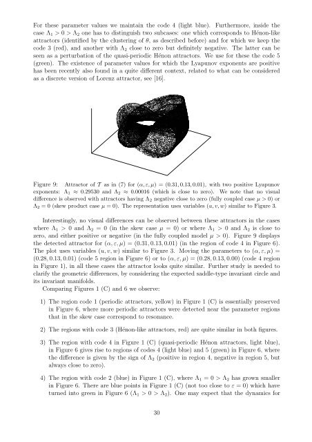
Figure 9: Attractor of T as in (7) for (α, ε, µ) = (0.31, 0.13, 0.01), with two positive Lyapunov
exponents: Λ 1 ≈ 0.29530 and Λ 2 ≈ 0.00016 (which is close to zero). We note that no visual
difference is observed with attractors having Λ 2 negative close to zero (fully coupled case µ > 0) or
Λ 2 = 0 (skew product case µ = 0). The representation uses variables (u, v, w) similar to Figure 3.
Interestingly, no visual differences can be observed between these attractors in the cases
where Λ 1 > 0 and Λ 2 = 0 (in the skew case µ = 0) or where Λ 1 > 0 and Λ 2 is close to
zero, and either positive or negative (in the fully coupled model µ > 0). Figure 9 displays
the detected attractor for (α, ε, µ) = (0.31, 0.13, 0.01) (in the region of code 4 in Figure 6).
The plot uses variables (u, v, w) similar to Figure 3. Moving the parameters to (α, ε, µ) =
(0.28, 0.13, 0.01) (code 5 region in Figure 6) or to (α, ε, µ) = (0.28, 0.13, 0.00) (code 4 region
in Figure 1), in all these cases the attractor looks quite similar. Further study is needed to
clarify the geometric differences, by considering the expected saddle-type invariant circle and
its invariant manifolds.
Comparing Figures 1 (C) and 6 we observe:
1) The region code 1 (periodic attractors, yellow) in Figure 1 (C) is essentially preserved
in Figure 6, where more periodic attractors were detected near the parameter regions
that in the skew case correspond to resonance.
2) The regions with code 3 (Hénon-like attractors, red) are quite similar in both figures.
3) The region with code 4 in Figure 1 (C) (quasi-periodic Hénon attractors, light blue),
in Figure 6 gives rise to regions of codes 4 (light blue) and 5 (green) in Figure 6, where
the difference is given by the sign of Λ 2 (positive in region 4, negative in region 5, but
always close to zero).
4) The region with code 2 (blue) in Figure 1 (C), where Λ 1 = 0 > Λ 2 has grown smaller
in Figure 6. There are blue points in Figure 1 (C) (not too close to ε = 0) which have
turned into green in Figure 6 (Λ 1 > 0 > Λ 2 ). One may expect that the dynamics for
30