Chaos and quasi-periodicity in diffeomorphisms of the solid torus

iterates in Ij 1 1
. These iterates are sorted with respect to θ and the oscillations of the x variable
are computed in the subintervals of the form [j 1 /10+k/100, j 1 /10+(k+1)/100], k = 0, 1, . . . 9.
Let Ij 2 1 ,j 2
be the subinterval with largest oscillation. This process is repeated as many times
as needed, until the maximal slope, based on the computed points, is no longer changing in a
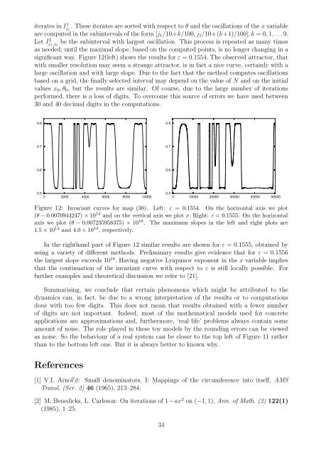
significant way. Figure 12(left) shows the results for ε = 0.1554. The observed attractor, that
with smaller resolution may seem a strange attractor, is in fact a nice curve, certainly with a
large oscillation and with large slope. Due to the fact that the method computes oscillations
based on a grid, the finally selected interval may depend on the value of N and on the initial
values x 0 , θ 0 , but the results are similar. Of course, due to the large number of iterations
performed, there is a loss of digits. To overcome this source of errors we have used between
30 and 40 decimal digits in the computations.
0.8
0.8
0.7
0.7
0.6
0.6
0.5
0 2000 4000 6000 8000 10000
0.5
0 10000 20000 30000 40000 50000
Figure 12: Invariant curves for map (38). Left: ε = 0.1554. On the horizontal axis we plot
(θ − 0.0070944247) × 10 14 and on the vertical axis we plot x. Right: ε = 0.1555. On the horizontal
axis we plot (θ − 0.007235958375) × 10 16 . The maximum slopes in the left and right plots are
1.5 × 10 12 and 4.0 × 10 14 , respectively.
In the righthand part of Figure 12 similar results are shown for ε = 0.1555, obtained by
using a variety of different methods. Preliminary results give evidence that for ε = 0.1556
the largest slope exceeds 10 18 . Having negative Lyapunov exponent in the x variable implies
that the continuation of the invariant curve with respect to ε is still locally possible. For
further examples and theoretical discussion we refer to [21].
Summarising, we conclude that certain phenomena which might be attributed to the
dynamics can, in fact, be due to a wrong interpretation of the results or to computations
done with too few digits. This does not mean that results obtained with a fewer number
of digits are not important. Indeed, most of the mathematical models used for concrete
applications are approximations and, furthermore, ‘real life’ problems always contain some
amount of noise. The role played in these toy models by the rounding errors can be viewed
as noise. So the behaviour of a real system can be closer to the top left of Figure 11 rather
than to the bottom left one. But it is always better to known why.
References
[1] V.I. Arnol ′ d: Small denominators, I: Mappings of the circumference into itself, AMS
Transl. (Ser. 2) 46 (1965), 213–284.
[2] M. Benedicks, L. Carleson: On iterations of 1−ax 2 on (−1, 1), Ann. of Math. (2) 122(1)
(1985), 1–25.
34