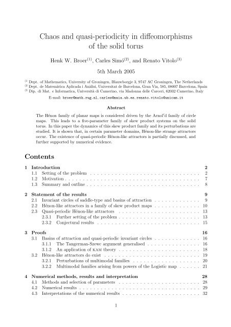
Chaos and quasi-periodicity in diffeomorphisms of the solid torus

Chaos and quasi-periodicity in diffeomorphisms
of the solid torus
Henk W. Broer (1) , Carles Simó (2) , and Renato Vitolo (3)
5th March 2005
(1 Dept. of Mathematics, University of Groningen, Blauwborgje 3, 9747 AC Groningen, The Netherlands
(2 Dept. de Matemàtica Aplicada i Anàlisi, Universitat de Barcelona, Gran Via, 585, 08007 Barcelona, Spain
(3 Dip. di Mat. e Informatica, Università di Camerino, via Madonna delle Carceri, 62032 Camerino, Italy
E-mail: broer@math.rug.nl, carles@maia.ub.es, renato.vitolo@unicam.it
Abstract
The Hénon family of planar maps is considered driven by the Arnol ′ d family of circle
maps. This leads to a five-parameter family of skew product systems on the solid
torus. In this paper the dynamics of this skew product family and its perturbations are
studied. It is shown that, in certain parameter domains, Hénon-like strange attractors
occur. The existence of quasi-periodic Hénon-like attractors is partially discussed, and
further supported by numerical evidence.
Contents
1 Introduction 2
1.1 Setting of the problem . . . . . . . . . . . . . . . . . . . . . . . . . . . . . . . 2
1.2 Motivation . . . . . . . . . . . . . . . . . . . . . . . . . . . . . . . . . . . . . . 7
1.3 Summary and outline . . . . . . . . . . . . . . . . . . . . . . . . . . . . . . . . 8
2 Statement of the results 9
2.1 Invariant circles of saddle-type and basins of attraction . . . . . . . . . . . . . 9
2.2 Hénon-like attractors in a family of skew product maps . . . . . . . . . . . . . 10
2.3 Quasi-periodic Hénon-like attractors . . . . . . . . . . . . . . . . . . . . . . . 13
2.3.1 Further setting of the problem . . . . . . . . . . . . . . . . . . . . . . . 13
2.3.2 Conjectural results . . . . . . . . . . . . . . . . . . . . . . . . . . . . . 15
3 Proofs 16
3.1 Basins of attraction and quasi-periodic invariant circles . . . . . . . . . . . . . 16
3.1.1 The Tangerman-Szewc argument generalised . . . . . . . . . . . . . . . 16
3.1.2 An application of kam theory . . . . . . . . . . . . . . . . . . . . . . . 18
3.2 Hénon-like attractors do exist . . . . . . . . . . . . . . . . . . . . . . . . . . . 19
3.2.1 Perturbations of multimodal families . . . . . . . . . . . . . . . . . . . 20
3.2.2 Multimodal families arising from powers of the Logistic map . . . . . . 21
4 Numerical methods, results and interpretation 28
4.1 Methods and selection of parameters . . . . . . . . . . . . . . . . . . . . . . . 28
4.2 Numerical results . . . . . . . . . . . . . . . . . . . . . . . . . . . . . . . . . . 29
4.3 Interpretations of the numerical results . . . . . . . . . . . . . . . . . . . . . . 32
1

1 Introduction
Since the 1990’s several mathematical characterisations have been found concerning the structure
of strange attractors in families of maps. A basic example is provided by the Hénon
attractor [18], occurring in the family of maps
H a,b :
2 → 2 , (x, y) ↦→ (1 − ax 2 + y, bx), (1)
where a and b are real parameters. Benedicks and Carleson [2, 3] proved that there exists
a set of parameter values S, with positive Lebesgue measure, such that for all (a, b) ∈ S
the Hénon map H a,b (1) has a strange attractor coinciding with the closure Cl (W u (p)) of
the unstable manifold of a saddle fixed point p. Here Cl (−) denotes the topological closure.
Similar techniques were then used to prove occurrence of strange attractors in parametrised
families of maps, near homoclinic tangencies in two or higher dimensions [26, 32, 36, 39],
and near tangencies in the saddle-node critical case [14]. See [42] for a general set-up to
prove existence of strange attractors with one positive Lyapunov exponent in families of twodimensional
maps. The strange attractors considered in these references are called Hénonlike
[14, 26, 39].
1.1 Setting of the problem
In this paper we study certain model map families, searching these for Hénon-like attractors
as well as for so-called quasi-periodic Hénon-like attractors. A basic model for this study is
the family of maps of the solid torus 2 × ¡ 1 , where ¡ 1 = /¢ is the circle, given by
⎛ ⎞
x
⎛
⎞
1 − (a + ε sin(2πθ))x 2 + y
⎝y⎠ ↦→ ⎝
θ
bx
θ + α + δ sin(2πθ)
⎠ , (2)
where both (ε, δ) are perturbation parameters. This map is a skew product perturbation of
the Hénon map (1) by the Arnol ′ d family [1]
A α,δ : ¡ 1 → ¡ 1 , θ ↦→ θ + α + δ sin(2πθ). (3)
of maps of ¡ 1 . First let us consider the uncoupled situation where ε = 0. The dynamics of
the Arnol ′ d family is globally well-known and that of the Hénon family is partially known.
They are organised in the respective (α, δ)- and (a, b)-parameter planes, see Figure 1. For the
Arnol ′ d family in the (α, δ)-plane there is a countable union of resonance tongues with nonempty
interior, corresponding to hyperbolic periodic dynamics. In the complement, which
is of positive measure, we find quasi-periodic dynamics [1, 13]. See Figure 1 (A). Similarly,
for the Hénon family in the (a, b)-plane there exists a countable union of strips of non-empty
interior corresponding to hyperbolic periodic dynamics. In the complement a set of positive
measure corresponds to strange attractors [3]. Most of the strips are extremely narrow and
only become visible when they intersect another strip of the same period in such a way that
a “crossroad area” is created [4]. See Figure 1 (B).
Remark 1. Figure 1 is mostly obtained by numerical computation of Lyapunov exponents
[35]. Figure 1 (B) uses the origin as initial point, which can land either in a periodic sink, or on
a strange attractor or can escape ‘to infinity’. Notice that, due to multistability other initial
points can tend to different attractors. Moreover, some of the periodicity strips are connected
to windows of sinks of the Logistic family as this occurs for b = 0. The interpretation of the
results in Figure 1 (C) is given in Section 4.
2

1
0.8
0.6
(A)
0.4
0.2
0
0 0.1 0.2 0.3 0.4 0.5
0.6
0.5
0.4
(B)
0.3
0.2
0.1
0
0.2
1 1.2 1.4 1.6 1.8 2
0.15
(C)
0.1
0.05
0
0.2 0.25 0.3 0.35 0.4
Figure 1: (A) Organisation of the (α, δ)-parameter plane of the Arnol ′ d family (3) by resonance
tongues, containing an open set with periodic dynamics (indicated in black). The remaining parameter
values (indicated in white) form a nowhere dense set of positive measure with quasi-periodic
dynamics. (B) Organisation of the (a, b)-parameter plane of the Hénon family (1) by strips with
periodic dynamics and crossroad areas (in red). A complement of positive measure contains strange
attractors (in green). The upper right part of the diagram (in white) corresponds to escape. (C) Diagram
of map (2) in the (α, ε)-plane, for a = 1.25, b = 0.3 and δ = 0.6/(2π). Visible are: domains
which can be interpreted has having periodic attractors (code 1, yellow), quasi-periodic attractors
(code 2, blue), Hénon-like attractors (code 3, red) and quasi-periodic Hénon-like attractors (code 4,
light blue). For more details see the main text, in particular Sections 1.3, 2.3 and 4.
3

For map (2) there are at least four combinations of the Arnol ′ d and Hénon families for
the uncoupled case ε = 0 that correspond to parameter domains of positive measure.
1. We start considering the case where the Hénon family is in a periodic attractor, so
where the (maximal) Lyapunov exponent Λ H < 0.
(a) In the most simple case, both constituents are in a hyperbolic periodic attractor,
compare with Figures 1 (A) and (B). The corresponding (maximal) Lyapunov
exponents Λ A and Λ H are both negative. In the solid torus
2 ¡ × 1 this also gives
a hyperbolic periodic attractor, that is persistent for |ε| ≪ 1.
(b) In a second case, the Arnol ′ d family is quasi-periodic, while the Hénon family is
in a periodic attractor. Now Λ A = 0, while Λ H < 0. The corresponding uncoupled
dynamics in the solid torus again is a normally hyperbolic quasi-periodic attractor,
which by centre manifold theory [20] and by kam theory [5, 6] has certain
persistence properties for |ε| ≪ 1.
2. In the two remaining cases the Hénon family is in a strange attractor, so with Λ H > 0.
This attractor is the closure Cl (W u (Orb(p))) of the unstable manifold of a periodic
saddle point. (Below we shall be more precise.) We have to distinguish two cases.
¡ ¡
(a) In the former of these, the Arnol ′ d family is in a periodic attractor, so with Λ A < 0,
and the product system has a Hénon-like attractor. It is the main aim of this paper
to show the persistence of this attractor for |ε| ≪ 1. For illustrations see Figure
2. Here we shall focus on small values of b, which allows us to rescale our model
(2) by ε. In fact we shall consider a sufficiently smooth family of skew-product
diffeomorphisms T α,δ,a,ε given by
⎛ ⎞
x
⎛
⎞
1 − ax 2 + εf
T α,δ,a,ε :
2 × 1 → 2 × 1 , ⎝y⎠ ↦→ ⎝
θ
εg
A α,δ (θ)
⎠ . (4)
Here (α, δ, a, ε) are parameters, while f and g are functions of (a, x, y, θ, ε, α, δ).
For 0 ≤ δ < (1/2π) and α ∈ [0, 1], the map A α,δ is a diffeomorphism of the circle
¡ 1 . We perturb away from cases where (α, δ) is in one of the resonance tongues,
see Figure 1 (A).
(b) In the latter case, where the Arnol ′ d family is quasi-periodic, so with Λ A = 0, the
uncoupled product dynamics is quasi-periodic Hénon-like, i.e., on an attractor of
the form Cl (W u (C )) , where C is a quasi-periodic invariant circle of saddle-type,
again compare Figure 1 (A). We conjecture that this phenomenon is persistent for
|ε| ≪ 1, but have only partial results in this direction, supported by numerics.
For illustrations see Figures 3 and 4.
The Lyapunov diagram in Figure 1 (C) strongly suggests that all four cases occur in parameter
sets of positive measure. More concretely, case 1(a) corresponds to code 1; case 1(b) to code
2; case 2(a) to code 3, and case 2(b) to code 4.
Our interest is with phenomena that are persistent under small perturbations, both within
the skew product setting and beyond this. To this end, we also consider a more general class
of families defined as follows. First let
K = (K 1 , K 2 ) :
2 → 2 (5)
4

1
θ
(A)
1
θ
(B)
replacements
0.5
PSfrag replacements
0.5
(A)
0
-1
0
x
1
-0.4
0
y
0.4
0
-1
0
x
1 -0.4
Figure 2: Hénon-like strange attractors of the model family (2) for (α, δ) in Arnol ′ d tongues of
periods two and three. (A) Parameters are fixed at a = 1.3, b = 0.3, ε = 0.2, (α, δ) = (0.51, 0.116).
(B) Same as (A) for α = 0.33793.
0
y
0.4
w
PSfrag replacements
v
u
Figure 3: Quasi-periodic Hénon-like strange attractor of the model family (2). Parameter values
are fixed at a = 1.85, b = −0.2, δ = 0, α = ( √ 5 − 1)/2, ε = 0.1. For a better visualisation of the
folds, the plot is given in the variables (u, v, w), where u = (r + 4) cos(θ), v = (r + 4) sin(θ), with
r = x cos(θ) + 10y sin(θ), and w = −x sin(θ) + 10y cos(θ).
be a dissipative (i.e., area contracting) diffeomorphism, that is sufficiently smooth. Next,
denote by R α : ¡ 1 → ¡ 1 the rigid rotation R α (θ) = θ + α. Then we define the family
P α,ε :
2 × ¡ 1 → 2 × ¡ 1 , (x, y, θ) ↦→ ( K 1 (x, y) + P 1 , K 2 (x, y) + P 2 , θ + α + P 3
)
, (6)
of diffeomorphisms, where P j , for j = 1, . . . , 3, is a smooth function of (x, y, θ, α, ε) such
that P j = 0 for ε = 0. Notice that the model (6) is not a skew product, but that there
is full coupling of the two constituents. A hyperbolic fixed point p of K (5) corresponds
to a normally hyperbolic invariant circle C α,0 = {p} ¡ × 1 for the map P α,ε at ε = 0. By
normal hyperbolicity the circle C α,0 is persistent under small perturbations [20, Theorem
1.1]. Similar remarks go for the case where p is a hyperbolic periodic point. In the sequel we
shall use this both for the case where p is a saddle and where p is a sink.
For numerical illustrations and discussion, a concrete version of (6) is used. It consists of
5

0.4
0
-0.4
y
rag replacements
x
-0.8
θ
(A)
0 0.2 0.4 0.6 0.8 1
0.4
0
rag replacements
-0.4
y
-0.8
θ
(A)
x
-2 -1 0 1
(B)
Figure 4:(A) Quasi-periodic Hénon-like attractor of the model family (2), projection on the (θ, y)-
plane. Parameter values are fixed at a = 0.8, b = 0.4, δ = 0, α = ( √ 5 − 1)/2, ε = 0.7, initial
conditions x 0 = 1.5, y 0 = 0, θ 0 = 0. (B) Same as (A), projection on the (x, y)-plane (in grey, in the
background). ‘Slices’ of the attractor for 2πθ ∈ [0.1 × j, 0.1 × j + 0.001], j = 0, 1, . . . , 62, are plotted
in black.
6

eplacements
2
1
0
-1
x
z
-2
(A)
P (Σ)
PSfrag replacements Σ
0.8 1 1.2 1.4
(A)
Σ
P (Σ)
x
z
x
ỹ
1.938
1.932
1.926
(B)
1.24 1.3 1.36 1.42
Figure 5: (A) Strange attractor A of the Poincaré return map of a climatological system [9].
Compare with Figure 3. The attractor A is plotted with a ‘slice’ Σ and with the image of Σ under
the return map. The slice Σ contains all points with distance less that 0.0001 from the plane z = 0.
The image of Σ is magnified in the central box. (B) Slice Σ of the attractor A in (A), projection
on the (x, ỹ)-plane, with ỹ = y − 0.133 ∗ z.
¡ ¡
a perturbation of (2), where a coupling term in µy is added to the angle dynamics:
⎛ ⎞
x
⎛
⎞
1 − (a + ε sin(2πθ))x 2 + y
T = T α,δ,a,b,ε,µ :
2 × 1 → 2 × 1 , ⎝y⎠ ↦→ ⎝
θ
bx
θ + α + δ sin(2πθ) + µy
⎠ , (7)
depending on the six parameters (α, δ, a, b, ε, µ).
1.2 Motivation
Quasi-periodic Hénon-like attractors have been conjectured to occur in diffeomorphisms of
3 = {x, y, z}, obtained as Poincaré return maps for a climatological model [9, 10, 41],
compare the attractor A displayed in Figure 5. Examination of a cross-section Σ of the
attractor (magnified in Figure 5 (B)) suggests that A is contained in a two-dimensional
manifold which is folded onto itself, in analogy with the structure of the Hénon attractor [18].
This manifold supposedly is the unstable manifold W u (C ) of a quasi-periodic invariant circle
C of saddle type. To illustrate the dynamics inside A we computed the image of the slice Σ
under the return map. This yields a folded curve looking like a planar Hénon attractor.
Remark 2. Also we mention that the occurrence of strange attractors which look similar
to Figure 4 (A) is observed in [28, 15, 17, 22, 29]. Although most of these studies deal with
endomorphisms of the interval forced by a rigid rotation in a skew product way, and some of
them have negative Lyapunov exponents (beyond the one trivially equal to zero), there may
be a relationship with the present approach. See Sections 2.3 and 4 for further discussion.
The theoretical knowledge of attractors in higher dimension is limited. As positive exceptions
to this we mention Viana [39, 40], Tatjer [36] and Wang & Young [42]. The Hénon-like
attractors found in the present paper, to some extent, also belong to this domain. In this
sense one may say that the understanding of the quasi-periodic Hénon-like attractor is a
next step in this research program. A more detailed discussion and further motivation of the
search for quasi-periodic Hénon-like attractors is postponed to Section 2.3.
7

1.3 Summary and outline
We summarise the remainder of this paper, also explaining its organisation. First in Section 2
the results are presented, where all longer proofs are postponed to Section 3. The contents of
Section 2 are related as follows to the subdivision regarding model (2) as given in Section 1.1.
Numerical examples beyond the skew product model (2), as well as details on methods and
on the interpretation of the results, are given in Section 4.
Normally hyperbolic invariant circles
In Section 2.1 we start considering the more general context of the fully coupled family (6).
A hyperbolic periodic point p, for ε = 0 corresponds to a normally hyperbolic invariant circle
C .
We start with the case where p is a saddle-point, so where C normally is of saddle type as
well. Theorem 2 asserts that now, under quite general conditions, the closure Cl (W u (C )) of
the unstable manifold of C attracts an open set. In the families (6) and (2) this corresponds
to an open set of parameter values. Note that the attracting set Cl (W u (C )) is not minimal
if C carries Morse-Smale dynamics. In this situation, the case 2(a) of Section 2 is partially
covered.
Next, if p is a hyperbolic periodic point of the family (6), Theorem 3 guarantees that C
is quasi-periodic for a parameter set of positive measure. If p is a saddle-point, in combination
with the previous paragraph, we partially cover case 2(b) of Section 1.1 for the family
(2). However, if p is a periodic sink, it follows that C is a quasi-periodic attractor, which
completely covers case 1(b) of Section 1.1.
In the case where p is a sink and C carries Morse-Smale dynamics, for the general setting
of (6), the minimal attractors are periodic. For the family (2) this completely covers case
1(a) of Section 1.1.
Persistence of normally hyperbolic invariant circles generally follows by [20, Theorem 1.1].
Theorem 2 is based on a result by Tangerman and Szewc, see [31, Appendix 3]. Our proof
of Theorem 3 applies standard kam Theory, see [6, 5].
The cases where Λ H > 0
We now deal with the cases where the Hénon family is in a strange attractor. The main
mathematical contents of this paper are formulated in Theorem 4 (in Section 2.2), which
deals with the scaled skew product model (4). Here we establish the existence of Hénon-like
strange attractors, which completely covers case 2(a) of Section 1.1 in suitable parameter
ranges. For completeness, in Section 2.2 technical definitions of ‘strange’, ‘Hénon-like’, etc.,
are included; compare with [14, 26, 39]. The proof of Theorem 4 is based on [14, Theorem
5.2].
Finally, in Section 2.3 we deal with the remaining case, both for the skew product system
(4) and for the more general system (6). Here we touch upon the existence of quasi-periodic
Hénon-like attractors. Lemma 7 implies that in the product case ε = 0 a topologically
transitive attractor occurs, having a dense set of orbits with a positive Lyapunov exponent.
Regarding its persistence for |ε| ≪ 1, our conjectures and mostly computer suggested.
Acknowledgements
The authors are indebted to Henk Bruin, Àngel Jorba, Marco Martens, Vincent Naudot,
Floris Takens, Joan Carles Tatjer and Marcelo Viana for valuable discussion. The first author
8

is indebted to the Departament de Matemàtica Aplicada i Anàlisi, Universitat de Barcelona,
for hospitality and the last two authors are indebted to the Department of Mathematics,
University of Groningen, for the same reason. The research of C.S. has been supported by
grants DGICYT BFM2003-09504-C02-01 (Spain) and CIRIT 2001 SGR-70 (Catalonia). The
computing cluster HIDRA of the UB Group of Dynamical Systems have been widely used.
We are indebted to J. Timoneda for keeping it fully operative.
2 Statement of the results
As announced before, our results are formulated in the next subsections, while proofs are
given in Sections 3.1 and 3.2.
2.1 Invariant circles of saddle-type and basins of attraction
We first consider maps F of the solid torus
2 × ¡ 1 obtained by perturbing the product of a
¡
¡ ¡
planar map times a rotation on 1 . Assuming that the planar map has a saddle fixed point
with a transversal homoclinic point, it is proved that the map F has an attractor contained
inside Cl (W u (C )).
To this end we generalise an unpublished result of Tangerman and Szewc, see [31, Appendix
3], where we are in the general context of the family P α,ε : 2 × 1 → 2 × 1 , see
(6).
Proposition 1. (normally hyperbolic invariant circle) Suppose that K has a hyperbolic
fixed point p = (x 0 , y 0 ). Then for all α ∈ [0, 1] the map P α,0 has a normally hyperbolic
invariant circle C α,0 = {p} × ¡ 1 . The manifold C α,0 is r-normally hyperbolic for all integers
r with 1 ≤ r ≤ n. Moreover, for all r < n there exists an ε r > 0 such that for all ε < ε r
and all α ∈ [0, 1], P α,ε has a normally hyperbolic invariant circle C α,ε of class C r , which is
C r -close to C α,0 .
Proof: The dynamics of P α,0 on C α,0 is parallel with rotation number α. This implies that
C α,0 is an r-normally hyperbolic invariant manifold for all r ≤ n and, therefore, it is of
class C n . So C α,0 (as well as its stable and unstable manifolds), is persistent under C n -small
perturbations. This directly follows from [20, Theorem 1.1].
Proposition 1 allows us to construct a basin of attraction with nonempty interior for the
invariant set Cl (W u (C α,ε )), provided that p is a saddle point, while the one-dimensional
unstable manifold W u (p) ⊂ 2 of the map K, see (5), does not escape to infinity. For
(x, y, θ) ∈ 2 × ¡ 1 , denote by ω(x, y, θ) the ω-limit set of (x, y, θ) under P α,ε .
Theorem 2. (attractor contained in Cl (W u (C ))) Fix integers n and r such that
n ≥ 2 and 1 ≤ r < n. Choose ε < ε r as in Proposition 1 and let α ∈ [0, 1]. Suppose that
K : 2 → 2 is of class C n and satisfies:
1. K has a saddle fixed point p ∈ 2 and a transversal homoclinic point q ∈ W s (p)∩W u (p).
2. K is uniformly dissipative: there exists κ < 1 such that |det(DK(x, y))| ≤ κ for all
(x, y) ∈ 2 .
3. W u (p) is contained in a bounded subset of 2 .
9

Then there exists an ε ∗ < ε r such that for all ε < ε ∗ there exists an open, nonempty bounded
set U ⊂
2 × ¡ 1 such that for all (x, y, θ) ∈ U
ω(x, y, θ) ⊂ Cl (W u (C α,ε )) . (8)
Remark 3. By taking iterates of the map P α,ε , Theorem 2 can be adapted to the case
where p is a saddle periodic point. In this context we have the inclusion (8), where C α,ε is a
periodically invariant circle, i.e. a circle which is invariant under some iterate of P α,ε .
Under the conditions of Theorem 2, the invariant set Cl (W u (C α,ε )) attracts all orbits with
initial state in an open set U. This holds for an open set of ε-values. In general, however,
Cl (W u (C α,ε )) is not an attractor, since it might be non-topologically transitive. This occurs,
for example, if Cl (W u (C α,ε )) contains a periodic attractor.
In the next Theorem we prove that at least the circle C α,ε is quasi-periodic (and, hence,
topologically transitive) for a set of parameter values having large relative measure.
Theorem 3. (normally hyperbolic quasi-periodic circles) Let P α,ε be a C n -family
of diffeomorphisms as in (6), where n ≥ 5. Choose ε r as in Proposition 1. Then there exists
an ε ∗∗ < ε r such that for all ε < ε ∗∗ the following holds.
1. There exists a set D ε ⊂ [0, 1] with Lebesgue measure meas(D ε ) > 0 such that for
α ∈ D ε the restriction of P α,ε to the circle C α,ε is smoothly conjugate to an irrational
rigid rotation.
2. meas(D ε ) tends to 1 for ε → 0.
Proofs of Theorems 2 and 3 are given in Section 3.1.
Theorem 3, as happens with Theorem 2, has a direct analogue for the case where p is
a hyperbolic periodic point. The Theorems will be applied both for the case where p is
a periodic saddle and a periodic sink. In the latter case we prove the existence of quasiperiodic
attractors for positive measure in parameter space, as described in the case 2(b) of
Section 1.1. Again see Figure 1 (C). This situation corresponds to points with code 2, in
blue.
A complementary situation regarding Theorem 3 occurs when the dynamics on C α,ε is
of Morse-Smale type, compare with the resonance tongues of Figure 1 (A). In that case,
for Λ H < 0, the attracting set Cl (W u (C α,ε )) of system (6) contains a hyperbolic periodic
attractor as described in case 1(a) of Section 1.1. Again compare with Figure 1 (C), points
with code 1, in yellow. In the next section, for the skew product system (4) we show that in
the case where Λ H > 0, the set Cl (W u (C α,ε )) contains a Hénon-like attractor, which covers
the case 2(a) of Section 1.1, compare with Figure 1 (C), points with code 3, in red.
2.2 Hénon-like attractors in a family of skew product maps
By Theorem 2, the set Cl (W u (C )) is attracting under quite general circumstances. As may
be clear from the previous paragraph, in general Cl (W u (C )) does not have to be topologically
transitive, in which case it is not considered an attractor. (For precise definitions see below.)
However, in the particular case of map (2), we show that Cl (W u (C )) contains Hénon-like
attractors. We first recall a few basic definitions regarding strange attractors, suited to our
purposes.
Definition 1. [14, 26, 39] Let F : M → M be a C 1 -diffeomorphism, where M is an
m-dimensional smooth manifold.
10

1. An F -invariant set A ⊂ M is called topologically transitive if there exists a point
z ∈ A such that the orbit Orb(z) = {F j (z)} j≥0 of z under F is dense in A .
2. A set A ⊂ M is called an attractor if it is topologically transitive, compact, F -invariant
and if the stable set (basin of attraction) W s (A ) has nonempty interior.
3. An attractor A is called strange if there exist constants κ > 0, λ > 1, a dense orbit
Orb(z) ⊂ A and a vector v ∈ T z M such that
‖DF n (z)v‖ ≥ κλ n for n ≥ 0.
4. The attractor A is called Hénon-like if there exist a saddle periodic orbit Orb(p) =
{p, F (p), . . . , F n (p)}, a point z in the unstable manifold W u (Orb(p)), constants κ > 0,
λ > 1, and tangent vectors v, w ∈ T z M, with w ≠ 0, such that
where Cl(·) denotes topological closure.
i) A = Cl (W u (Orb(p))) , (9)
ii) Orb(z) is dense in A , (10)
iii) ‖DF n (z)v‖ ≥ κλ n for n ≥ 0, (11)
iv) ‖DF n (z)w‖ → 0 as n → ±∞, (12)
In particular, Hénon-like attractors are strange, since by conditions (10) and (11) they admit
a dense orbit with a positive Lyapunov exponent. Moreover, Hénon-like attractors are nonuniformly
hyperbolic; indeed, by condition (12) they contain critical points, that is, points
belonging to a dense orbit for which a nonzero tangent vector w exists, which is contracted
both by positive and by negative iteration of the derivative DF .
We now come to the main result of the present paper, regarding the occurrence of Hénonlike
strange attractors in the scaled skew product family (4). First we recall that the restriction
of (4) to ¡ 1 is the Arnol ′ d family of circle maps (3). Moreover, the map (4) is a
generalisation of the planar Hénon-like families considered in [26, 39]. The latter are families
of planar diffeomorphisms, which are C 3 -small perturbations of the Logistic family
Q a : → , x ↦→ 1 − ax 2 . (13)
The x- and y-components of T α,δ,a,ε also depend on the circle dynamics by the perturbative
terms f and g. The only requirement on f and g is that their C 3 -norms are bounded on
compact sets. Occurrence of Hénon-like attractors is proved in the family T α,δ,a,ε for all
parameter values belonging to a set of positive (Lebesgue) measure. For all values in this
set, the parameters (α, δ) are such that the dynamics of the Arnol ′ d family A α,δ (3) is of
Morse-Smale type: there exist periodic points θ s and θ r ¡ in 1 , such that θ s is attracting and
θ r repelling for A α,δ . By A q/n we denote the open resonance tongue in the (α, δ)-plane where
these periodic points have rotation number q/n [1, 13] and the width of the tongue in α
behaves as δ n [8], compare with Figure 1 (A). The parameter space under consideration is
the set of all (α, δ, a, ε) ∈
4 such that
α ∈ [0, 1], δ ∈ [ 0, 1/(2π) ) , a ∈ [0, 2], |ε| < 1. (14)
The attractors A we obtain, coincide with the closure of the one-dimensional unstable manifold
A = Cl (W u (Orb(p))) ,
where p = (x 0 , y 0 , θ s ) ∈
2 ¡ × 1 belongs to a hyperbolic periodic orbit of saddle type. For
the statement of the result we need a few definitions and notations.
11

Definition 2. 1. A map M : J → J, where J ⊂ is an interval, is called topologically
mixing if for any open intervals J 1 , J 2 ⊂ J there exists n 0 such that
M n (J 1 ) ∩ J 2 ≠ ∅ for all n ≥ n 0 .
2. The interval K a = [Q 2 a (0), Q a(0)] is called the core or the restrictive interval of the
Logistic family Q a (13).
It is well-known that Q a ([0, 1]) = Q a (K a ) = K a for all a, where K a is the core of Q a (13),
see e.g. [24, Section II.5]. For a given integer n > 1, denote by Φ(n) the set of all integers q
such that q and n are relatively prime, where 1 ≤ q < n. For n = 1 we put Φ(n) = {1}.
Theorem 4. (Hénon-like attractors in (4)) Choose a ∗ ∈ (1, 2) such that the quadratic
map Q a ∗ in (13) is topologically mixing on its core K = [1 − a ∗ , 1] and its critical point c = 0
is preperiodic. Let n ≥ 1 be an integer. There exist a periodic point p 0 of the n-th iterate Q n a ∗
and positive constants ¯ε n , ā n and χ n such that the following holds.
1. For all (α, δ, a, ε) as in (14), with
(α, δ) ∈ ∪ q∈Φ(n) Cl ( A q/n) , |a − a ∗ | < ā n , |ε| < ¯ε n (15)
the map T α,δ,a,ε has a saddle periodic point p, which is the analytic continuation of p 0
and such that the unstable manifold W u (Orb(p)) is one-dimensional.
2. For all (α, δ, ε) as in (15) there exists a set S α,δ,ε with
S α,δ,ε ⊂ [a ∗ − ā n , a ∗ + ā n ],
meas(S) > χ n
such that for all a ∈ S α,δ,ε the closure Cl (W u (Orb(p))) is a Hénon-like attractor of
T α,δ,a,ε .
Corollary 5. The set of parameter values for which T α,δ,a,ε has a Hénon-like attractor contains
the set
S = ⋃ n∈
{
(α, δ, a, ε) | (α, δ) ∈ ∪q∈Φ(n) Cl ( A q/n) , |ε| < ¯ε n , a ∈ S α,δ,ε
}
,
and the set S has positive Lebesgue measure
meas(S) ≥ 2
∞∑
¯ε n χ n
n=1
∑
q∈Φ(n)
meas A q/n .
Our proof of Theorem 4 is given in Section 3.2. It is based on a result of Díaz-Rocha-Viana [14,
Theorem 5.2], and relies on the following facts:
1. For (α, δ) inside any tongue A q/n , the asymptotic dynamics of T α,δ,a,ε is described by
an O(ε)-perturbation of the n-th iterate Q n a .
2. For all n the map Q n a is a generic n-modal family, in the sense of [14, Section 5.2],
also see the definition given in Section 3.2. To show this, we use that Q a ∗ is a Misiurewicz
map [25], and, therefore, it is Collet-Eckmann (see e.g. [24, Section V.4]). See
Section 3.2 for details.
12

Notice that the family (2) takes the form (4) after a rescaling y ↦→ √ |b|y and by choosing b =
O(ε). Therefore, by restricting the parameter δ to sufficiently small values, both Theorem 4
and Theorem 2 may be applied to (2).
Corollary 6. Let a ∗ and p 0 satisfy the hypotheses of Theorem 4. Then there exists a positive
measure set of parameter values such that the family (2) has Hénon-like attractors, contained
in the closure of the unstable manifold of a periodically invariant circle.
Proof: Take a ∗ and p 0 as in the hypotheses of Theorem 4. Then for all δ and for ε and b
sufficiently small, Theorem 4 applies. Moreover, for (ε, δ) = (0, 0) the circle C = {p 0 } × ¡ 1 is
periodically invariant under map (2). In particular, the conditions of Theorem 2 are satisfied
for b sufficiently small, since:
1. The periodic point (p 0 , 0) of H a,0 has an analytic continuation ¯p(b) for all b sufficiently
small, and p 0 is chosen such that ¯p(b) has transversal homoclinic points, see Proposition
12.
2. det(DH a,b (x, y)) = b;
3. The unstable manifold of all periodic points of H a,b is bounded for b sufficiently small,
since the invariant manifolds depend continuously on the map [26, Prop. 7.1].
So for (ε, δ, b) sufficiently small, the conclusions of Theorem 2 hold.
Two attractors occurring in the family (2) are shown in Figure 4 (A) and (B), for (α, δ) in an
Arnol ′ d resonance tongue of period two and three, respectively. Also compare with Figure
1 (C), points with code 3, in red. It is to be noted that the Hénon-like character of these
attractors for larger values of b and ε remains conjectural.
2.3 Quasi-periodic Hénon-like attractors
We start with a further setting of the problems regarding quasi-periodic Hénon-like attractors,
in the skew product model family (2).
2.3.1 Further setting of the problem
The present paper has been partially motivated by the problem to find a diffeomorphism F
with a strange attractor A such that
A = Cl (W u (C )) , (16)
where C is an F -invariant circle of saddle type with irrational rotation number, so with quasiperiodic
dynamics. In this context, the role of the saddle periodic orbit in (9) is played by
a quasi-periodic invariant circle of saddle type. By analogy with the definition of Hénon-like
strange attractors (see Section 2.2), we are led to the following definition.
Definition 3. Let F : M → M be a C 1 -diffeomorphism, where M is an m-dimensional
smooth manifold. We say that the attractor A is quasi-periodic Hénon-like if there exist
1. A quasi-periodic invariant circle C of saddle type such that A = Cl (W u (C )) .
2. A point x ∈ A such that Orb(x) is dense in A and
3. a dense set Z ⊂ A and constants κ > 0, λ > 1 such that for all z ∈ Z there exist
vectors v, w ∈ T z M such that conditions (11) and (12) hold.
13

The definition mimics the positive Lyapunov exponents and non-uniform hyperbolicity requirements
in the definition of Hénon-like attractors and also asks for transitivity. As usual
similar definitions can be given with F replaced by a power F k .
Returning to the skew product context of the model family (2), in the Arnol ′ d family A α,δ
we fix parameter values (α, δ) such that the dynamics of A α,δ is quasi-periodic. Recall that
the set of all such (α, δ) has positive measure and is nowhere dense [5, Chap. 1]. Next choose
parameter values a and b such that the Hénon map (1) has a Hénon-like strange attractor
A ′ , coinciding with the closure of the unstable manifold of a saddle fixed point p. Also recall
that, according to [2, 3, 26], such (a, b) form a set of positive measure. Then, at ε = 0 the
map (2) has an attractor A = A ′ × ¡ 1 coinciding with the closure of the unstable manifold
of the quasi-periodic saddle-type invariant circle {p}ס 1 . It may be clear that requirement 3
of Definition 3 is satisfied by taking Z = Orb(z) × ¡ 1 , where z is a point satisfying properties
4 ii), iii) and iv) in Definition 1 of Hénon-like attractors.
Next, to prove that in the product case we obtain a quasi-periodic Hénon-like attractors
only item 2 in Definition 3 has to be verified. This is done in the following lemma.
Lemma 7. (Transitivity of (2), uncoupled) Let T be a dissipative C 1 -diffeomorphism
in an open subset U ⊂
2 such that
1. T has a hyperbolic fixed point p of saddle-type.
2. The closure of the unstable manifold of p is an Hénon-like strange attractor A ′ .
Let R α : x ↦→ x + α mod 1 a rotation over angle α ∈ (0, 1) \
has a dense orbit in A = A ′ ¡ × 1 .
. Then the product F = T × R
Proof: We claim that it is sufficient to prove the following:
(∗) Given two open sets U, V in A , there exists k ∈ ¡ such that F k (U) ∩ V ≠ ∅.
Indeed, given ε > 0 there is a finite number of open sets V j , j ∈ J, of the form V j =
V j ′ × (s j − ε, s j + ε) that cover A , where V j ′ ⊂ 2 is an open ball of radius ε. Let U 0 = U.
Assuming (∗), it follows that F k 1
(U 0 ) intersects V 1 for some k 1 ¡ ∈ . Define U 1 as the image
under F −k 1
of this intersection. This process can be repeated for all j ∈ J. After this we
restart the whole process with ε replaced by ε/2, ε/4, ε/8, . . ., ε/2 m , . . . , each time obtaining
an open set U m such that U m ⊂ U m+1 . The intersection ∩ m∈ U m gives an initial point for a
dense orbit as desired.
Next, let us prove (∗). Without loss of generality, assume that U = U ′ × (r − δ, r + δ) and
V = V ′ × (s − ε, s + ε) for some δ, ε > 0, where U ′ , V ′ are open sets in A ′ . First, for fixed
ε > 0 we note that given r, s ¡ ∈ 1 there exists an increasing sequence {n 1 , n 2 , . . .} such that
R n j
α (r) ∈ (s − ε, s + ε), where 0 < n 1 < N and n j+1 − n j < N for all j, with N independent of
r and s. As W u (p) is dense in A ′ , there exists a point q ′ ∈ W u (p) ∩ V ′ . Consider a preimage
u = T −l (q ′ ) such that u and its first N iterates are close to p. By continuity, there are
open sets Z 0 , Z 1 , . . . , Z N
around u, T (u), . . . , T N (u) whose images under T l , T l−1 , . . . , T l−N
are contained in V ′ .
Now, there exists a point x ∈ U ′ ∩ W u (p) belonging to a dense orbit and also having a
positive Lyapunov exponent, such that T m (x) ∈ Z 0 for some m ∈ ¡ . It is no restriction to
assume that, for some m ∈ ¡ , the image T m (U ′ ) intersects all Z j , j = 0, 1, 2, . . . , N. Indeed,
in the other case the Lyapunov exponent could not be positive.
Since T l−j (Z j ∩ T m (U ′ )) ⊂ V ′ for j = 0, . . . , N, one has
T l+m−j (U ′ ) ∩ V ′ ≠ ∅ (17)
14

for all j = 0, . . . , N. To arrange that some of the iterates Rα
l+m−j (r) lie inside the interval
(s − ε, s + ε), observe that l + m is in between two consecutive values n i and n i+1 for some
n i as above. This implies that there exists j with ≤ j ≤ N such that l + m − j = n i , which,
together with (17), yields that T l+m−j (U) ∩ V ≠ ∅.
0.2
0.15
0.1
0.05
0
0.2 0.25 0.3 0.35 0.4
Figure 6: Diagram of the fully coupled system (7) in the (α, ε)-plane, for a = 1.25, b = 0.3, µ = 0.01
and δ = 0.6/(2π). According to the values of the Lyapunov exponents, we interpret as follows:
domains of periodic attractors (code 1, yellow), of quasi-periodic attractors (code 2, blue), of Hénonlike
attractors (code 3, red) and of ‘quasi-periodic Hénon-like’ attractors (codes 4, light blue, and
5, green). For more details see Section 2.3 and Section 4.
2.3.2 Conjectural results
Numerical experiments with the map (2) suggest that attractors like A persist for small (and
perhaps, not so small) values of (ε, δ). See figures 3 and 4. Figure 1 (C) gives evidence that
quasi-periodic Hénon-like attractors occur in a relatively large part of the parameter plane
(code 4, light blue). In this numerical context, quasi-periodic Hénon-like are indicated by
the fact that one positive, one negative, and one zero Lyapunov exponent is detected. We
assume that the Lyapunov exponents are ordered as
Λ 1 ≥ Λ 2 ≥ Λ 3 .
A remarkable difference between the skew-product case (2) and the fully coupled case (7) is
that a zero Lyapunov exponent practically never occurs, compare Figure 6 and see Section 4.2.
Indeed, any small perturbation µ ≠ 0 has the effect of shifting the value of Λ 2 away from
zero. Its modulus remains small, but the sign may be either positive or negative, where both
cases occur. Plots of the attractors visually look the same in the three cases Λ 2 = 0, Λ 2 < 0
and Λ 2 > 0, when µ is small and the other parameters are kept fixed. It remains to be
clarified which dynamical and geometrical properties characterise the strange attractors in
each of the three cases. In any case, it seems that the way in which the invariant manifolds
of an invariant circle are folded, plays an essential role.
15

PSfrag replacements
p
U ′
∂ s
q
c
∂ u
d
Figure 7: Segments ∂ s and ∂ u of the stable and unstable manifold, respectively, of a saddle fixed
point p bound a region U, see text for more explanation.
Remark 4. 1. We used the family (7) for the figures, expecting that it is sufficiently rich
for our purposes.
2. When comparing the Figures 1 (C) and 6, the main difference is that in the second
case there is no significant occurrence of Λ 2 = 0. Still we expect that in all cases the
attractor is the closure Cl (W u (C )) of a quasi-periodic invariant circle C of saddle-type.
3. It seems that in the skew case (2), the phenomenon of an attractor with Λ 1 = 0 and
Λ 2 < 0, which is not an invariant circle is somewhat related to ‘nonchaotic strange
attractors’, compare with [28, 15, 17, 22, 29]. See also Section 4.3 for further discussion
on this topic.
Interestingly, tiny perturbations away from the skew case seemingly give rise to a quasiperiodic
Hénon-like attractor, so with Λ 1 > 0.
3 Proofs
3.1 Basins of attraction and quasi-periodic invariant circles
In this section we give proofs of Theorem 2 (next section) and Theorem 3 (Section 3.1.2).
3.1.1 The Tangerman-Szewc argument generalised
Let K : 2 → 2 be a dissipative diffeomorphism having a saddle fixed point p = (x 0 , y 0 ).
Suppose the stable and unstable manifolds W s (p) and W u (p) intersect transversally at the
homoclinic point q ∈ W s (p) ∩ W u (p), see Figure 7. Also assume that W u (p) is bounded as a
subset of
2 . The Tangerman-Szewc Theorem (see e.g. [31, Appendix 3]) states that the basin
of attraction of the closure of W u (p) contains the open region U ′ bounded by the two arcs
∂ s ⊂ W s (p) and ∂ u ⊂ W u (p) with extremes p and q, see Figure 7. This argument is used to
prove existence of strange attractors (in particular, with non-trivial basin of attraction) near
homoclinic tangencies of a saddle fixed point of a dissipative diffeomorphism, cf. [26, 39, 42].
We first prove Theorem 2 for ε = 0. This is a straightforward generalisation of the
above Tangerman-Szewc Theorem. For small ε, the result is obtained by using persistence of
normally hyperbolic invariant manifolds [20, Theorem 1.1] and two transversality lemmas.
16

Proof of Theorem 2. Consider the circle C α = C α,0 , invariant under map P α,0 in (6). The
manifolds W u (C α ) and W s (C α ) are given by W u (p) × ¡ 1 and W s (p) × ¡ 1 , respectively. They
intersect transversally at a circle H = {q} × ¡ 1 , consisting of points homoclinic to C α .
Consider the two arcs ∂ s ⊂ W s (p) and ∂ u ⊂ W u (p) with extremes p and q (Figure 7).They
bound an open set U ′ ⊂
2 . Define D s and D u to be the portions of stable, and unstable
manifold of C α , respectively, given by
D s = ∂ s × ¡ 1 ⊂ W s (C α ) and D u = ∂ u × ¡ 1 ⊂ W u (C α ).
Both surfaces D s and D u are compact, and their union forms the boundary of the open region
U = U ′ × 1 , which ¡ is topologically a solid torus.
The volume of U decreases under iteration of P α,0 . Denoting by meas(·) the Lebesgue
measure both on 2 and on 2 × 1 , due to condition 2 ¡ in Theorem 2 we have
∫
∫
meas(Pα,0 n (U)) = 2π dxdy = 2π |det DK n | dxdy ≤ 2πκ n meas(U ′ ).
K n (U ′ )
U ′
This implies that the forward evolution of every point (x, y, θ) ∈ U approaches the boundary
of P n α,0 (U): dist ( P n α,0(x, y, θ), ∂P n α,0(U) ) → 0 as n → +∞.
Indeed, suppose that this does not hold. Then there exists a ϱ > 0 such that for all n there
exists N > n such that the ball with centre Pα,0(x, N y, θ) and radius ϱ > 0 is contained inside
Pα,0 N (U). But this would contradict the fact that meas(P α,0 n (U)) → 0 as n → +∞.
The boundary of Pα,0 n (U) also consists of two portions of stable and unstable manifold of
C :
∂Pα,0 n (U) = P α,0 n (Ds ) ∪ Pα,0 n (Du ).
The diameter of P n α,0(D s ) tends to zero as n → +∞, because all points in D s are attracted
to the circle C α . Since W u (C α ) is bounded, all evolutions starting in U are bounded and
approach W u (C α ), that is,
dist(P n α,0 (x, y, θ), P n α,0 (Du )) → 0 as n → +∞
for all (x, y, θ) ∈ U. This implies that ω(x, y, θ) ⊂ Cl (W u (C α )) for all (x, y, θ) ∈ U.
To extend this result to small perturbations P α,ε of P α,0 , the following transversality
lemmas are used.
Lemma 8. [33, Chap. 7] Consider a map f : V → M, where V and M are C r -
differentiable manifolds and f is C r . Suppose V is compact, W ⊂ M is a closed C r -
submanifold and f is transversal to W at V (notation: f ⋔ W ). Then f −1 (W ) is a C r -
submanifold of codimension codim V (f −1 (W )) = codim M (W ). Further suppose that there is
a neighbourhood of f(∂ V ) ∪ ∂ W disjoint from f(V ) ∩ W , where ∂ V and ∂ W are the boundaries
of V and W . Then any map g : V → M, sufficiently C r -close to f, is also transversal to W ,
and the two submanifolds g −1 (W ) and f −1 (W ) are diffeomorphic.
Lemma 9. [19, Section 3.2] Let V 1 , V 2 , and M be C r -differentiable manifolds and consider
two diffeomorphisms f i : V i → M, i = 1, 2. Then f 1 ⋔ f 2 if and only if f 1 × f 2 ⋔ ∆,
where f 1 × f 2 : V 1 × V 2 → M × M is the product map and ∆ ⊂ M × M is the diagonal:
∆ = {(y, y) | y ∈ M}.
Fix r ¡ ∈ and take ε < ε r , where ε r is given in Proposition 1. Then the map P α,ε has
an r-normally hyperbolic invariant circle C α,ε of saddle type. Furthermore, the manifolds
W u (C α,ε ), W s (C α,ε ), and C α,ε are C r -close to W u (C α ), W s (C α ), and C α . We now show
17

that the two manifolds W u (C α,ε ), W s (C α,ε ) still intersect transversally. To apply Lemma 8
we restrict to two suitable compact subsets A u ⊂ W u (C α ) and A s ⊂ W s (C α ) as follows.
Consider the segments pc ⊂ W u (p) and pd ⊂ W s (p) in Figure 7. Define
A u = pc × ¡ 1 , A s = pd × ¡ 1 .
In this way, the circle H is the intersection of the manifolds A u and A s , bounded away from
their boundaries. Consider the inclusions i : A u → M and j : A s → M. By the closeness of
W u (C α ) to W u (C α,ε ) there exists a C r -diffeomorphism h : A u → A u ε ⊂ W u (C α,ε ) such that
the map i is C r -close to i ε ◦ h, where i ε : A u ε → M is the inclusion [30, Section 2.6]. Similarly,
there exists a diffeomorphism k : A s → A s ε ⊂ W s (C α,ε ) such that the map j is C r -close j ε ◦ k,
where j ε : A s ε → M is the inclusion. By Lemma 9 the map i × j : Au × A s → M × M is
transversal to the diagonal ∆. For ε small, the map (i ε ◦ h) × (j ε ◦ k) : A u × A s → M × M is
C r -close to i × j:
A u × A s i×j
−−−→ M × M
⏐
h×k↓
A u ε × A s i ε×j ε
ε −−−→ M × M.
Since ∆ is closed and A u × A s is compact, Lemma 8 implies that there exists an ε ∗ , with
0 < ε ∗ < ε r , such that (i ε ◦ h) × (j ε ◦ k) ⋔ ∆ for ε < ε ∗ . Furthermore, the submanifolds
(i × j) −1 (∆) and
(
(iε ◦ h) × (j ε ◦ k) ) −1
(∆)
are diffeomorphic. We also have that ( (i ε ◦ h) × (j ε ◦ k) ) −1 (∆) is diffeomorphic to A u ε ∩ As ε ,
and (i × j) −1 (∆) = A u ∩ A s = H .
This shows that the intersection H ε = A u ε ∩ As ε is diffeomorphic to H . Define Du ε as the
part of W u (C α,ε ) bounded by the invariant circle C α,ε and the circle of homoclinic points H ε .
Define Dε s = k(D s ) similarly. Then the manifolds Dε u ⊂ W u (C α,ε ) and Dε s ⊂ W s (C α,ε ) form
the boundary of an open region U ⊂ M homeomorphic to a torus. By the closeness of the
perturbed manifolds W s (C α,ε ) and W u (C α,ε ) to the unperturbed W s (C ) and W u (C ), both U
and W u (C α,ε ) are bounded. Also notice that P α,ε is dissipative: by taking ε ∗ small enough,
we ensure that |det(DF (x, y, θ))| < ˜c < 1 for all ε < ε ∗ and (x, y, θ) in U. Therefore, all
forward evolutions beginning at points (x, y, θ) ∈ U remain bounded. Like in the first part
of the proof, one has
ω(x, y, θ) ⊂ Cl (W u (C α,ε ))
for all (x, y, θ) ∈ U, α ∈ [0, 1] and ε < ε ∗ .
3.1.2 An application of kam theory
So far, we did not discuss the dynamics in the saddle invariant circle C α,ε of map P α,ε
in (6). Generically, the dynamics on C α,ε is of Morse-Smale type. In this case, the circle
consists of the union of the unstable manifold of some periodic saddle. Theorem 3 describes
a complementary case, for which the dynamics is quasi-periodic. Fix τ > 2 and define the
set of Diophantine frequencies D γ by
{
D γ = α ∈ [0, 1] |
∣ α − p }
q ∣ ≥ γq−τ for all ¡ p, q ∈ , q ≠ 0 , (18)
where γ > 0. Since we will apply a version of the KAM Theorem holding for non-conservative,
finitely differentiable systems (see [5, Chap. 5] and [6]), a certain amount of smoothness of
the circle C α,ε is needed, depending on the Diophantine condition specified in (18). Therefore
we require that the perturbed family of maps P α,ε is C n , for n large enough.
18

Proof of Theorem 3. Consider map P α,0 in (6), and let p = (x 0 , y 0 ) be a saddle fixed point
of the diffeomorphism K. The invariant circle C α,0 = {p} × ¡ 1 of P α,0 can be trivially seen
as a graph over ¡ 1 :
C α,0 = { (x 0 , y 0 , θ) | θ ∈ ¡
1 } .
Fix r ¡ ∈ large enough and ε < ε r , where ε r is taken as in Proposition 1. By the C r -closeness
of C α,0 and C α,ε (Proposition 1), the circle C α,ε of P α,ε can be written as a C r -graph ¡ over 1 :
C α,ε = { (x ε (θ), y ε (θ), θ) ∈ 2 × ¡ 1 | θ ∈ ¡
1 } , (19)
where x ε ¡ : 1 → , x ε (θ) = x 0 + O(ε), and similarly for y ε (θ). So the restriction of P α,ε to
C α,ε has the following form
P α,ε
∣
∣Cα,ε
: C α,ε → C α,ε , P α,ε (θ) = θ + α + εg ε (x 0 , y 0 , θ, α) + O(ε 2 ).
By (19), we may consider P α,ε as a map on ¡ 1 . Fix γ > 0, τ > 3 and take D γ as in (18). For
α ∈ D γ , the map P α,ε can be averaged repeatedly over the circle, putting the θ-dependency
into terms of higher order in ε, compare [8, Proposition 2.7] and [11, Section 4]. After such
changes of variables, P α,ε is brought into the normal form
P α,ε (θ) = θ + α + c(α, ε) + O(ε r+1 ).
In fact, it is convenient to consider α as a variable, and to define the cylinder maps
P ε : ¡ 1 × [0, 1] → ¡ 1 × [0, 1], P ε (θ, α) = (P α,ε (θ), α)
R : ¡ 1 × [0, 1] → ¡ 1 × [0, 1],
R(θ, α) = (R α (θ), α),
where R α : ¡ 1 → ¡ 1 is the rigid rotation of an angle α. We now apply a version of the KAM
Theorem, holding for non-conservative, finitely differentiable systems (see e.g. [5, Chap. 5]
and [6]), to the family of diffeomorphisms P ε . There exists an integer m with 1 ≤ m < r and
a C m -map
Φ ε : ¡ 1 × [0, 1] → ¡ 1 × [0, 1], Φ ε (θ, α) = (θ + εA(θ, α, ε), α + εB(α, ε)), (20)
such that the restriction of Φ ε to ¡ 1 × D γ makes the following diagram commute:
1 × ¡
R
D γ −−−→ 1 × D ¡ γ
↑ ↑
Φ ⏐⏐
ε Φ ⏐⏐
ε
1 × D ¡
P ε
γ −−−→ 1 × D ¡ γ .
The differentiability of Φ ε restricted to ¡ 1 × D γ is of Whitney type. Since P α,ε
∣
∣Cα,ε
is C m -
conjugate to a rigid rotation on ¡ 1 , the circle C α,ε is in fact C m . This proves parts 1 and 2
of the Theorem.
Furthermore, the constant γ in (18) can be taken equal to ε r . This gives that the measure
of the complement of D γ in [0, 1] is of order ε r as ε → 0.
3.2 Hénon-like attractors do exist
Our proof of Theorem 4 is based on a result of Díaz-Rocha-Viana [14]. We begin by stating
this result.
19

3.2.1 Perturbations of multimodal families
Two definitions from [14, Section 5.2] are introduced now. For more information about the
terminology, we refer to [24, Sections II.5, II.6].
Definition 4. Let J ⊂ be a compact interval. Fix d ≥ 1, k ≥ 3, a ∗ ∈ , and an interval
of parameter values U = [a − , a + ], with a ∗ ∈ Int U. A C k -family of maps M a : J → J, with
a ∈ U, is called a d-family if it satisfies the following conditions:
1. Invariance: M a ∗(J) ⊂ Int(J);
2. Nondegenerate critical points: M a ∗ has d critical points {c 1 , . . . , c d } def
= Cr M a ∗ that satisfy
M ′′
a ∗(c i) ≠ 0 for all i and M a ∗(c i ) ≠ c j for all i, j;
3. Negative Schwarzian derivative: SM a ∗ < 0 for all x ≠ c i , where
Sf(x) = f ′′′ (x)
f ′ (x) − 3 ( ) f ′′ 2
(x)
;
2 f ′ (x)
4. Topological mixing: There exists an interval J ′ ⊂ Int(J) such that M a ∗(J) = M a ∗(J ′ ) = J ′
and such that for any open intervals J 1 , J 2 in J ′ there exists n 0 such that
M n a ∗(J 1) ∩ J 2 ≠ ∅ for all n ≥ n 0 ;
5. Preperiodicity: for each 1 ≤ i ≤ d there exists m i such that p i = M m i
a ∗ (c i) is a (repelling)
periodic point of M a ∗;
6. Genericity of unfolding: For all c i ∈ Cr M a ∗, denote by c i (a) and p i (a) the continuations
of c i and p i , respectively, for a close to a ∗ . Then
d (
M
m i
a
da
(c i(a)) − p i (a) ) ≠ 0 at a = a ∗ .
Next we introduce the notion of η-perturbation of a d-family M a , with a ∈ U and d ≥ 1 fixed.
Definition 5. Fix σ > 0 and consider the family M a obtained by extending M a as follows:
M a : J × I σ → J × I σ ,
M a (x, y) def
=(M a (x), 0). (21)
Also denote by M the map
M : U × J × I σ → J × I σ ,
M(a, x, y) def
= M a (x, y) = (M a (x), 0).
Given a C k -family of diffeomorphisms
for a k ≥ 3, denote by G its extension
G a : J × I σ → J × I σ , a ∈ J,
G : U × J × I σ → J × I σ ,
G(a, x, y) def
= G a (x, y).
Then G is called a η-perturbation of the d-family {M a } a if
‖M − G‖ C k ≤ η,
where ‖·‖ C k denotes the C k -norm over U × J × I σ .
20

The following proposition is used in the sequel to prove existence of Hénon-like attractors for
the map (2). See [2, 3, 26, 32, 37, 39, 42] for similar results.
Proposition 10. [14, Theorem 5.2] Let {M a } a be a d-family and p a periodic point of
M a ∗. Then there exist η > 0, ā and χ > 0 such that, given any η-perturbation {G a } a of
{M a } a the following holds.
1. For all a with |a − a ∗ | < ā the map G a has a periodic point p a which is the continuation
of the periodic point (p, 0) of the map M a in (21).
2. There exists a set S, contained in the interval [a ∗ − ā, a ∗ + ā] ⊂ U, with meas(S) > χ,
such that for all a ∈ S there exists z ∈ W u (p a ) satisfying:
(a) the orbit {G n a(z) | n ≥ 0} is dense in Cl (W u (Orb(p a )));
(b) G a has a positive Lyapunov exponent at z, i.e., there exist k > 0, λ > 1 and v ≠ 0
such that ‖DG n a(z)v‖ ≥ kλ n for all n ≥ 0;
(c) there exist w ≠ 0 such that ‖DG n a(z)w‖ → 0 as n → ±∞.
3.2.2 Multimodal families arising from powers of the Logistic map
The proof of Theorem 4, which we present in this section, is based on three facts. First,
suppose that a ∗ ∈ [0, 2] is such that the quadratic family Q a (x) = 1 − ax 2 in (13) is a d-
def
family in the sense of Definition 4, with d = 1. Then for all n ≥ 1 the family M a = Q n a
given by the n-th iterate of Q a is a d-family for some d ≤ 2 n . Second, for all η 1 > 0, the
composition of an η 1 -perturbation of Q a with an η 1 -perturbation of Q n a is an η 2-perturbation
of Q n+1
a , where η 2 = C(n)η 1 and C(n) is a positive constant depending on n. Third, for each
n > q ≥ 1 and for each (α, δ) ∈ A q/n , the asymptotic dynamics of T α,δ,a,ε is described by a
map that turns out to be an η-perturbation of the d-family M a , with η = O(ε). Moreover,
M a has a periodic point p such that its analytic continuation in the family T α,δ,a,ε possesses
a transversal homoclinic intersection. Application of Proposition 10 to the point p concludes
the proof.
In the next lemma we show that M a is a d-family. For each ã ∈ [0, 2) there exists a β > 0
such that for all a with a ∈ [0, ã] the interval J = [−1−β, 1+β] ⊂ satisfies Q a (J) ⊂ Int(J).
In the sequel, it is always assumed that the family Q a is defined on such an interval J, and
that the values of a we consider are such that Q a (J) ⊂ Int(J).
Lemma 11. Suppose a ∗ ∈ [0, 2) def
= U is such that the quadratic family
Q a : J → J, Q a (x) = 1 − ax 2
satisfies hypotheses 4 and 5 of Definition 4. Then for all n ≥ 1 there exists d ≥ 1 such that
the family
def
M a : J → J, M a = Q n a
is a d-family with d ≤ 2 n − 1 critical points.
Proof. Take a ∗ as above. We first prove the case n = 1, that is, Q a : J a → J a is a 1-family.
Conditions 1, 2, 3 of Definition 4 are obviously satisfied by Q a . Condition 6 will now be
proved. By conditions 4 and 5 (assumed by hypothesis), Q a ∗ is a Misiurewicz map [25], i.e.,
it has no periodic attractor and c ∉ ω(c), where c = 0 is the critical point of Q a ∗. Moreover,
21

y [24, Theorem III.6.3] the map Q a ∗ is Collet-Eckmann (see e.g. [24, Section V.4]), that is,
there exist constants κ > 0 and λ > 1 such that
∣ d
∣∣∣
∣dx a ∗(Q a ∗(c)) ≥ κλ n for all n ≥ 0. (22)
Therefore, by combining [38, Theorem 3] with the Collet-Eckmann condition (22) we get
lim
n→∞
d
da Qn a (c) | a=a ∗
d
dx Qn−1 a ∗ (Q a
∗(c))
> 0. (23)
Assume Q k a ∗(c) = p, with p periodic (and repelling) under Q a∗. By p(a) denote the continuation
of p for a close to a ∗ . Then, for all n sufficiently large,
d
da Qn a (c) | a=a ∗ = ∂Qn−k a
∂a
= ∂
∂a Qn−k a
= d da
(Qk a ∗(c)) | a=a ∗ +∂Qn−k a
∂x (Qk a ∗(c)) | d
a=a ∗
(p) | a=a ∗ + ∂
d
(p) | a=a ∗
(
Q
n−k
a (p(a)) ) + ∂
∂x Qn−k a
∂x Qn−k a ∗
da Qk a (c) | a=a ∗=
[
p(a) + Q
k
da
a (c) − p(a) ] | a=a ∗=
(p) d [
Q
k
da a (c) − p(a) ] | a=a ∗ .
(24)
The point Qa
n−k (p(a)) belongs to a hyperbolic periodic orbit, that varies smoothly with the
parameter a. Therefore, its derivative with respect to a (which is the first term in the last
equality) is uniformly bounded in n. On the other hand,
d
dx Qn−1 a ∗
(Q a ∗(c)) = ∂
∂x Qn−k a ∗
(p) d
dx Qk−1 a ∗
(Q a ∗(c)).
Therefore, by (22), (23), and (24) we conclude that
d
da
0 < lim
Qn a (c) | [
d
a=a ∗
n→∞ d
dx Qn−1 a (Q ∗ a ∗(c)) = da Q
k
a (c) − p(a) ] a=a ∗
d
dx Qk−1 a (Q ∗ a ∗(c)) . (25)
This proves that Q a satisfies condition 6 of Definition 4.
We now show that the n-th iterate M a of the quadratic map is a d-family for all n > 1
and for some d ≤ 2 n . For simplicity, we denote Q a ∗ by Q for the rest of this proof. Condition
1 holds for M a ∗ since it holds for Q a ∗. Condition 3 follows from the fact that the composition
of maps with negative Schwarzian derivative also has negative Schwarzian derivative, see
e.g. [24, II.6]. Condition 4 is obviously satisfied.
Condition 2 is now proved by induction on n, where the case n = 1 is obvious. Obviously,
the set Cr M a ∗ of critical points of M a ∗ has cardinality d ≤ 2 n − 1. Moreover,
Cr M a ∗ = Q ( −1 Cr Q n−1) n−1
⋃
∪ Cr Q = (Q −j )(Cr Q). (26)
Suppose that condition 2 holds for a given n ≥ 1. We first show that
j=0
(Q n+1 ) ′′ (x) ≠ 0 for all x ∈ Cr Q n+1 . (27)
By (26), if x ∈ Cr Q n+1 then either x = c, or Q(x) ∈ Cr Q n . If x = c then
(Q n+1 ) ′′ (x) = (Q n ) ′ (Q(c)) · (Q) ′′ (c). (28)
22

The second factor is nonzero. If the first factor is zero, then
0 = (Q n ) ′ (Q(c)) = Q ′ (Q n (c)) . . . Q ′ (Q(c)).
Therefore there exists j such that Q j (c) = c, so that c is an attracting periodic point of
Q. But this contradicts the fact that Q is Misiurewicz, so that (28) is nonzero. The other
possibility is that c ≠ x and Q(x) ∈ Cr Q n . In this case,
(Q n+1 ) ′′ (x) = (Q n ) ′′ (Q(x)) · Q ′ (x) 2 ,
which is nonzero. Indeed, Q ′ (x) ≠ 0, otherwise x = c. Moreover (Q n ) ′′ (Q(x)) ≠ 0 by the
induction hypotheses since the critical points of Q n are nondegenerate. This proves (27),
from which the first part of condition 2 follows.
We now prove, again arguing by contradiction, that
Q n+1 (x) ≠ y for all x, y ∈ Cr Q n+1 .
Suppose that there exist x, y ∈ Cr Q n+1 such that Q n+1 (x) = y. By (26) there exist i and j
such that Q i (x) = Q j (y) = c, where 0 ≤ i, j ≤ n. This would imply that
Q n+1+j−i (c) = Q j (Q n+1 (x)) = Q j (y) = c,
with n + 1 + j − i ≥ 1 and, therefore, c would be an attracting periodic point of Q, which is
impossible since Q is Misiurewicz. Condition 2 is proved.
To prove condition 5, fix y ∈ Cr M a ∗ and j ≥ 0 such that Q j (y) = c. Since c is preperiodic
for Q by hypothesis, there exists k ≥ 1 such that Q j+k (y) = p, where p is periodic under Q
with period u ≥ 1. The orbit of y under M a ∗ is, except for a finite number of initial iterates,
a subset of the orbit of p under Q. This shows that y is preperiodic for M a ∗.
To prove condition 6, take y ∈ Cr M a ∗, j, u, k and p ∈ J as in the proof of condition 5.
Then there exist integers l and m, with 0 ≤ l < u and m ≥ 1, such that
M m a ∗(y) = Qk+l (c) = Q l (p) ∈ Orb Q (p). (29)
By condition 5 (assumed by hypothesis) and by (29), the point z = Q l (p) is periodic (and
repelling) under M a ∗. Denote by y(a), z(a), and p(a) the continuations of y, z, and p,
respectively, for a close to a ∗ . In particular,
We have to show that
By the chain rule we get
d
da Ql+k a
Q j a (y(a)) = c and Ql a (p(a)) = z(a).
d
da [M m a (y(a)) − z(a)]| a=a ∗ ≠ 0. (30)
(c) ∣ a=a ∗
= ∂Ql a
∂a (Qk a (c))∣ ∣
a=a ∗
+ ∂Ql a
∂x (Qk a (c))∣ ∣
dQ k a
a=a ∗
da (c)| a=a
= ∗
= ∂Ql a ∗
∂a (p) + ∂Ql a ∗
∂x (p) dQk a ∗
da (c),
d
da Ql a(p(a)) ∣ a=a ∗
= ∂Ql a ∗
∂a (p) + ∂Ql a ∗
∂x (p) d da p(a∗ ),
where p = p(a ∗ ) = Q k a∗(c). Therefore,
d
da [M a m (y(a)) − z(a)]| a=a ∗ = d [
Q
k+l
a (c) − Q l
da
a(p(a)) ]∣ ∣
a=a ∗
=
= ∂Ql a ∗
∂x (p) d [
Q
k
da a (c) − p(a) ]∣ ∣
a=a ∗
.
[
The factor d da Q
k
a (c(a)) − p(a) ]∣ ∣
a=a ∗
is nonzero by (25). The same holds for the other factor,
otherwise p would be an attracting periodic point of Q a ∗. This proves inequality (30).
23

Proposition 10 does not provide a nontrivial basin of attraction for the closure Cl (W u (p a )).
We now show that, under the hypotheses of Theorem 4, there exists a periodic point p a for
which a nontrivial basin of attraction of Cl (W u (p a )) can be constructed. Therefore, in this
case Cl (W u (p a )) is a Hénon-like attractor.
Proposition 12. Consider the map {Ma ∗ } a = Q n a ∗, where Q a∗ satisfies the hypotheses of
Lemma 11. There exist a periodic point p of Q a ∗, and positive constants η, ā and χ such that
for any η-perturbation {G a } a of {M a } a = Q n a the following holds.
∗
1. For all a with |a − a ∗ | < ā the map G a has a periodic point p a which is the continuation
of the periodic point (p, 0) of the map M a in (21). Moreover, p a has a transversal
homoclinic intersection.
2. There exists a set S, contained in the interval [a ∗ − ā, a ∗ + ā] ⊂ U, with meas(S) > χ,
such that for all a ∈ S the set Cl (W u (Orb(p a ))) is a Hénon-like attractor of the map
G a .
Proof. To construct a non-trivial basin of attraction for Cl (W u (Orb(p a ))), it is sufficient
to find a periodic point p a of {G a } a that has a transversal homoclinic intersection. Then
the basin is provided by the Tangerman-Szewc Theorem (see Theorem 2 and subsequent
remark). Indeed, for all η sufficiently small, all η-perturbations of the map Q ∗ a are uniformly
dissipative. Moreover, the unstable manifold of p a is bounded, since it is bounded for Q a ∗
and since the invariant manifolds of a map depend continuously on the map [26, Prop. 7.1].
Therefore, the second part of the proposition follows from the first part, together with the
Tangerman-Szewc argument and Proposition 10.
To prove the first part, we claim that the map Q a ∗ has a periodic point p belonging to
a non-degenerate homoclinic orbit. Indeed, if the claim is true, then for η sufficiently small
and for a close to a ∗ , any η-perturbation of M a possesses a periodic point p a which is the
analytic continuation of p and such that p a has a transverse homoclinic intersection. The
latter property again follows from continuous dependence of the invariant manifolds on the
map [26, Prop. 7.1].
To prove the claim that Q a ∗ has a periodic point p belonging to a non-degenerate homoclinic
orbit we first show that there exists a point y 0 belonging to a degenerate homoclinic
orbit of Q a ∗. Since the critical point c of Q a ∗ is preperiodic, there exist positive integers k, h
such that Q k a ∗(c) = y 0 and y 0 is periodic with period h. The unstable manifold of any periodic
point of Q a ∗ is the whole core [1 − a ∗ , 1], since Q a ∗ is topologically mixing. Therefore, since
the critical point c belongs to W u (y 0 ), by taking preimages of c, a point q can be found such
that q ∈ Wloc u (y 0), Q l a∗(q) = c and Ql+k a (q) = y ∗ 0 for some integer l > 0. This means that y 0
belongs to a degenerate homoclinic orbit of Q a ∗.
We now prove that there exists a periodic point p of Q a ∗ having a non-degenerate homoclinic
orbit. This is achieved by examining a power of Q a ∗ for which all points of the orbit
of y 0 are fixed. Denote by Orb Qa ∗(y 0 ) = {y j | j = 0, . . . , h − 1} the orbit of y 0 , under Q a ∗,
where y j = Q j a ∗(y 0). Let m be the smallest multiple of h which is larger than k, and denote
f def
= Q m a ∗. Then, f(c) belongs to Orb Q a ∗(y 0 ) and all points y j are fixed for f. We can assume
that
f ′ (y j ) > 1 for all y j ∈ Orb Qa ∗(y 0 ) (31)
by taking f 2 instead of f if necessary.
Brouwer’s fixed point Theorem and continuity arguments ensure the existence of a fixed
point p of f, a critical point c ′ of f, and an interval I = (c ′ − δ, c ′ ) such that:
1. f ′ (p) < −1;
24

2. c ′ lies in the interval (y, p);
3. f is monotonically increasing in I;
4. p falls in the interval f(I).
The configuration of c, c ′ and y = f(c) within the graph of f looks like the sketch in Figure 8,
in the case y < c and f ′′ (c) > 0 (the other combinations of the sign of y − c and f ′′ (c) are
treated similarly). Since f is topologically mixing, the interval f(I) is contained in the
PSfrag replacements
p
f(c)
y
Figure 8: Graph of the map f from the proof of Proposition 12. Only the relevant branches of
the graph are plotted, in relation to the fixed points y, p and the critical points c and c ′ . See the
text for details.
unstable manifold of p. Therefore p belongs to a homoclinic orbit O.
Moreover, the homoclinic orbit O is non-degenerate. Indeed, if this was not the case, then
there would exist a critical point c ′′ of f belonging to O, so that f j (c ′′ ) = p for some j ¡ ∈ .
However, according to (26), and since c is preperiodic, the orbit of c ′′ under Q a ∗ eventually
lands inside Orb Qa ∗(y 0 ). It follows that p ∈ Orb Qa ∗(y 0 ), which is absurd, since f ′ (p) < −1
whereas (31) holds.
In the next lemma we show that the composition of a small perturbation of the map
Q a (x, y) = (Q a (x), 0) (we use here the notation of Definition 5) with a small perturbation of
Q n a (x, y) = (Qn a (x), 0) yields a small perturbation of Qn+1 a (x, y). As in Definition 5, denote by
Q, Q n : [0, 2]×J×I → J×I the functions Q(a, x, y) = (Q a (x), 0) and Q n (a, x, y) = (Q n a(x), 0),
respectively.
Lemma 13. For each η > 0 there exists a ζ > 0 such that for all F, G : [0, 2] × J × I → J × I
such that
‖G − Q‖ C 3 < ζ and ‖F − Q n ‖ C 3 < ζ, (32)
c ′
p
c
we have ∥ ∥G ◦ F − Q
n+1 ∥ ∥
C 3
< η. (33)
Proof. Write
G(a, x, y) =
( )
Qa (x) + g 1 (a, x, y)
g 2 (a, x, y)
and F (a, x, y) =
( )
Q
n
a (x) + f 1 (a, x, y)
.
f 2 (a, x, y)
25

Then
G ◦ F (a, x, y) −
( ) Q
n+1
a (x)
=
0
( −2a(f1 (a, x, y)) 2 − 2af 1 (a, x, y)Q n a (x) + g 1(
a, ˜f1 (a, x, y), f 2 (a, x, y) ) )
(
g 2 a, ˜f1 (a, x, y), f 2 (a, x, y) ) ,
where ˜f 1 (a, x, y) = Q n a(x) + f 1 (a, x, y). The C 3 -norm of the terms −2a(f 1 (a, x, y)) 2 and
−2af 1 (a, x, y)Q n a (x) is bounded by a constant times the C3 -norm of f 1 . We now estimate the
norm of ˜g 1 , defined by
˜g 1 (x 0 , x 1 , x 2 ) = g 1 (a, ˜f 1 (a, x, y), f 2 (a, x, y)).
Denote x 0 = a, x 1 = x, and x 2 = y. Then any second order derivative of ˜g 1 is a sum of terms
of the following type:
∂ 2 g 1 ∂ ˜f k ∂g 1 ∂ 2 ˜fk
,
,
∂x j x k ∂x l ∂x k ∂x j x l
where we put ˜f 2 = f 2 to simplify the notation. For the third order derivatives a similar
property holds. Since the C 3 -norm of ˜f k is bounded, we get that each term in the third order
derivative of ˜g 1 is bounded by a constant times the C 3 -norm of the g j . This concludes the
proof.
Proof of Theorem 4. The Theorem will be first proved for a ∗ < 2. The case a ∗ = 2
follows by choosing another value ā ∗ < 2 sufficiently close to 2. Fix a ∗ ∈ [0, 2) verifying the
hypotheses of Lemma 11. To begin with, we consider the case (α, δ) ∈ Int A 1 , the interior of
the tongue of period one. Then the Arnol ′ d family A α,δ on 1 has two hyperbolic fixed points
¡
θ1 s (attracting) and θ1 r (repelling), see [13, Section 1.14]. The θ-coordinate of both points
depends on the choice of (α, δ) ∈ Int A 1 . So for all ¡ θ ∈ 1 with θ ≠ θ1 r , the orbit of θ under
A α,δ converges to θ1 s . This means that the manifold
Θ 1 = { }
(x, y, θ) ∈ 2 × 1 | θ = θ1
s ¡ ⊂ 2 1
¡ ×
is invariant and attracting under T α,δ,a,ε . Denote by G a,1 the restriction of T α,δ,a,ε to Θ 1 :
G a,1 : Θ 1 → Θ 1 , (x, y, θ s 1 ) ↦→ (1 − ax2 + εf 1 , εg 1 , θ s 1 ),
where f 1 = f(a, x, y, θ s 1 , α, δ) and similarly for g 1. Since Q a ∗(J) ⊂ Int(J), there exists a
constant σ > 0 such that for all ε sufficiently small and all a close enough to a ∗ ,
G a,1 (J × I σ × {θ s 1 }) ⊂ Int(J × I σ × {θ s 1 })
T α,δ,a,ε
(
J × Iσ × (¡ 1 \ {θ r 1 })) ⊂ Int ( J × I σ × (¡ 1 \ {θ r 1 })) . (34)
Since Θ 1 is diffeomorphic to 2 , we consider G a,1 as a map of 2 . Then G a,1 , is an
η-perturbation of the quadratic family Q a (x), where η = O(ε). We now apply Proposition
12 to the family G a,1 . Let p 0 be the periodic point of M a ∗ as given by Proposition 12.
For all ε sufficiently small there exists a constant ā > 0 and a set S of positive Lebesgue
measure, contained in the interval [a ∗ − ā, a ∗ + ā], such that the following holds. For all
a ∈ [a ∗ − ā, a ∗ + ā], G a,1 has a saddle periodic point ¯p which is the continuation of the point
p 0 . Furthermore, for all a ∈ S the closure à = Cl ( W u (Orb Ga,1 (¯p)) ) is a Hénon-like attractor
of G a,1 contained inside Θ 1 . The point p = (¯p, θ1 s) is a saddle periodic point of the map T α,δ,a,ε,
and W u (Orb Tα,δ,a,ε (p)) = W u (Orb Ga,1 (¯p)) × {θ1 s}. Therefore A = Cl (W u (p)) = Ã × {θs 1 } is a
26
and

Hénon-like attractor of T α,δ,a,ε . Moreover, the basin of attraction of Cl (W u (p)) has nonempty
interior in 2 ¡ × 1 because of (34). This proves the claim for (α, δ) ∈ Int A 1 .
We pass to the case of higher period tongues. Suppose that (α, δ) ∈ Int A q/n , with
n > q ≥ 1. Then A α,δ has (at least) two hyperbolic periodic orbits
Orb(θ s 1 ) = {θs 1 , θs 2 , . . . , θs n }
Orb(θ r 1 ) = {θr 1 , θr 2 , . . . , θr n }
attracting, and
repelling.
For j = 1, . . . , n, denote by Θ j the manifold
Θ j = { (x, y, θ) ∈ 2 × ¡ 1 ) | θ = θ s j}
,
and define maps G j as the restriction of T α,δ,a,ε to Θ j :
G j : Θ j → Θ j+1 for j = 1, . . . , n − 1
G n : Θ n → Θ 1 ,
where
(x, y, θ1 s ) G j
↦→ (Q a (x) + εf j , εg j , θj+1 s ), for j = 1, . . . , n − 1
(x, y, θn) s ↦→ Gn
(Q a (x) + εf n , εg n , θ1).
s
Here, f j = f(a, x, y, θj s, α, δ). The manifold Θ 1 is invariant and attracting under the n-th
iterate of the map T α,δ,a,ε . For all (x, y, θ) in the complement of the set
the asymptotic dynamics is given by the map
{(x, y, θ) | θ ∈ Orb(θ r 1)} ,
def
G a,1,...n = G n ◦ G n−1 ◦ · · · ◦ G 1 .
Notice that each of the G j ’s is an η j -perturbation of the family Q a in the sense of Definition 5,
where η j = Bε and B can be chosen uniform on θj s (and, therefore, on (α, δ)).
Let p 0 be the periodic point of M a ∗ as given by Proposition 12. Then (p 0 , 0) is a saddle
periodic point for the map M a defined as in (21). Take η, ā, and χ as in Proposition 12. By
inductive application of Lemma 13 there exists an ¯ε > 0 depending on η and n such that
‖G a,1,...n − Q n ‖ C 3 < η,
for all (α, δ) ∈ Int A q/n and all |ε| < ¯ε. That is, G a,1,...n is an η-perturbation of M a for all q
with 1 ≤ q < n and all (α, δ, a, ε) with
(α, δ) ∈ A q/n ,
ε ∈ [−¯ε, ¯ε].
By Proposition 12 there exist an ā > 0 and a set S contained in the interval [a ∗ − ā, a ∗ + ā]
such that meas(S) ≥ χ and the following holds. For all a ∈ [a ∗ −ā, a ∗ +ā] the map G a,1,...,n has
a periodic point ¯p a which is the continuation of the periodic point (p 0 , 0) of M a . Moreover,
for all a ∈ S the closure à = Cl ( W u (Orb Ga,1,...,n (¯p a )) ) is a Hénon-like attractor of G a,1,...,n ,
contained inside Θ 1 .
To finish the proof, observe that p a = (¯p a , θ1 s) is a saddle periodic point of T α,δ,a,ε. The
set A = Cl ( W u (Orb Tα,δ,a,ε (p a )) ) is compact and invariant under T α,δ,a,ε . To show that A
has a dense orbit, fix parameter values as provided by Proposition 12 applied to G a,1,...n . Let
z ∈ Θ 1 a point having a dense orbit in à and satisfying properties (a)–(c) of Proposition 10.
Then given η > 0 and a point
q = T j α,δ,a,ε (q′ ) ∈ T j α,δ,a,ε (Ã × {θs 1 }), with 1 ≤ j ≤ n − 1,
27

there exists m > 0 such that dist(G m a,1,...n (z), q′ ) < η. By continuity of T j α,δ,a,ε
, for all ϱ > 0
there exists η > 0 such that
dist(T j α,δ,a,ε (q′′ ), T j α,δ,a,ε (q′ )) < ϱ for all q ′′ with dist(q ′′ , q ′ ) < η.
We conclude that for all ϱ > 0 there exists m > 0 such that
dist(T j α,δ,a,ε (Gm a,1,...n (z)), T j α,δ,a,ε (q′ )) = dist(T j+mn
α,δ,a,ε
(z), q) < ϱ.
This proves that the orbit of z under T α,δ,a,ε is dense in A . Properties (11) and (12) will now
be proved. Since G a,1,...,n = T n α,δ,a,ε on Θ 1, for any m ∈ ¡ and any z ∈ A we have
DT m α,δ,a,ε(z) = DT r α,δ,a,ε(G s a,1,...,n(z))DG s a,1,...,n(z),
where s = m mod n and r = m − s. Take z as above and a vector v = (v x , v y , 0) ∈ T z A
such that ∥ ∥ DG
s
a,1,...,n (z)v ∥ ∥ ≥ κλ s for all s, where κ > 0 and λ > 1 are constants. Since T r α,δ,a,ε
is a diffeomorphism for all r = 1, . . . , s − 1 and G s a,1,...,n(z) belongs to the compact set A for
all s ∈ ¡ , then there exists a constant c > 0 such that
∥ DT
m
α,δ,a,ε (z)v ∥ ∥ =
∥ ∥DT r
α,δ,a,ε (G s a,1,...,n (z))DGs a,1,...,n (z)v∥ ∥ ≥ c
∥ ∥DG s
a,1,...,n (z)v ∥ ∥ ,
where c is uniform in r. This proves property (11). Property (12) is proved similarly. This
shows that the closure Cl (W u (p a )) is a Hénon-like attractor of T α,δ,a,ε .
Remark 5. At the boundary of a tongue A q/n the Arnol ′ d family A α,δ has a saddle-node
periodic point θ 1 . However, the basin of attraction of Orb θ 1 still has nonempty interior, so
that the above conclusions hold for all (α, δ) in the closure Cl ( A q/n) .
4 Numerical methods, results and interpretation
4.1 Methods and selection of parameters
An important tool in the numerical exploration of dynamical systems consists of the computation
of Lyapunov exponents. Let us take a three-dimensional map T as before, with an
orbit {x j , j = 0, 1, 2, 3, . . .} . Following [35] we start with three independent tangent vectors,
of which the successive iterates under the derivative DT are computed, after some transient.
At each step (or after a given number of steps to speed up the process) the vectors are
orthonormalised.
It is useful to introduce Lyapunov sums, as we show now, for simplicity just considering the
iterates of one tangent vector. Let v 0 be the initial vector and write v n = DT n x 0
(v 0 ), i.e., the
tangent vector obtained after n iterations. Let ˆv n+1 = DT (x n )v n . Then v n+1 = ˆv n+1 /f n+1 ,
where f n+1 = ‖ˆv n+1 ‖. The Lyapunov sum then is defined as
LS n =
n∑
log(f j ). (35)
j=1
The Lyapunov exponent then is the average slope of the Lyapunov sum as n → ∞, that is,
the average of the logarithmic rates of increase of the length log(f j ).
In the numerical procedure estimates are produced of the average slope of LS n up to
some n for different values of n up to a maximal number of N iterates. The computations are
stopped before N iterates in case of escape, or if a periodic orbit is detected, or if different
28

estimates of the average coincide within a prescribed tolerance ρ. Typical values for N and
ρ in the present computations are 10 7 and 10 −6 , respectively.
One of the major problems is to detect values of the Lyapunov exponents very close to
zero. To this end several procedures have been proposed for obtaining the limit. Taking into
account that in the skew case the driving behaviour is quasi-periodic or periodic, a method of
successive filtering and fitting, similar to [7] can be suitable. Another method like MEGNO
(see [12] for an exposition and examples and [23] for a problem which requires a massive use
of it) is based of weighted averages and is very useful to detect small values of the Lyapunov
exponent. However, presently we simply use the Lyapunov sum (35) because this will help
to understand the behaviour of the system in some elementary cases, see Section 4.3.
To scan the behaviour of family T given by (7), several parameters have been fixed. We
chose δ = 0.6 such that resonant zones of the Arnol ′ d family are not too narrow, while still
most of the values of α give rise to quasi-periodic dynamics. Concerning the parameters a
and b of the Hénon family, we fixed b = 0.3 for historical reasons. It is the value used by
Hénon [18], and it is a good compromise between dissipation and visibility of the folds of
the unstable manifold. It was also used in [34], where the various attractors for this value
of b, for several values of a was studied, as well as the role of homoclinic and heteroclinic
tangencies (later on in the literature known as ‘crises’). The value a = 1.25 corresponds to a
periodic attractor of period 7 and allows for moderate values of ε in the forcing before escape
occurs. Finally we selected the values µ = 0 and µ = 0.01 for the skew and the fully coupled
case, respectively. Other values of µ have also been investigated, see Section 4.2.
Let Λ 1 ≥ Λ 2 ≥ Λ 3 be the three Lyapunov exponents. Since the family (7) is dissipative,
the role of Λ 3 is not very relevant. It can only help to decide, in case of periodic or quasiperiodic
attractors, whether the normal behaviour is of nodal type (Λ 2 > Λ 3 ) or of focal type
(Λ 2 = Λ 3 ). The major role is played by Λ 1 and Λ 2 and their position with respect to zero.
In some cases it is also interesting to use a complementary tool to help to decide whether
the attractor is quasi-periodic or has some ‘strange’ character. This occurs for small values
of ε. In the skew case µ = 0 one may expect to have a period 7 invariant curve if (α, δ) is in
the quasi-periodic domain and ε is sufficiently small. Similar behaviour can be expected for
µ > 0 small, for a large relative measure set in (α, δ).
The following method has been used. Consider iterates of T 7 , after some transient, and
sort them by the values of θ. If the attractor is an invariant curve (x(θ), y(θ)), then the
variation of the components (x, y) can be estimated from the iterates. This variation has to
remain bounded when the number of iterates increases and tend to the true variation (but see
Section 4.3 for some wrong interpretations of the results of these computations). To recognise
Hénon-like attractors for the fully coupled case µ > 0 a similar device is used. The values of
the angular component θ of the iterates, should cluster around the periodic orbit obtained in
the case µ = 0.
4.2 Numerical results
The diagrams in Figures 1 (C) and 6 are based on the values of the first two Lyapunov
exponents Λ 1 and Λ 2 . To be more precise, in Figure 1 (C) code 1 (yellow) corresponds to
0 > Λ 1 , code 2 (blue) to 0 = Λ 1 > Λ 2 , code 3 (red) to Λ 1 > 0 > Λ 2 and code 4 (light blue)
to Λ 1 > 0 = Λ 2 . Typically we considered a Lyapunov exponent as equal to zero whenever
|Λ j | < 10 −5 , j = 1, 2.
In Figure 6 a new case appears, namely where Λ 1 > Λ 2 > 0. Here the value of Λ 2 is
small but definitely positive. It occurs for some regions of the (α, ε) parameter plane which,
in the skew case µ = 0 of Figure 1 (C) seemingly show quasi-periodic Hénon-like attractors.
29

For these parameter values we maintain the code 4 (light blue). Furthermore, inside the
case Λ 1 > 0 > Λ 2 one has to distinguish two subcases: one which corresponds to Hénon-like
attractors (identified by the clustering of θ, as described before) and for which we keep the
code 3 (red), and another with Λ 2 close to zero but definitely negative. The latter can be
seen as a perturbation of the quasi-periodic Hénon attractors. We use for these the code 5
(green). The existence of parameter values for which the Lyapunov exponents are positive
has been recently also found in a quite different context, related to what can be considered
as a discrete version of Lorenz attractor, see [16].
Figure 9: Attractor of T as in (7) for (α, ε, µ) = (0.31, 0.13, 0.01), with two positive Lyapunov
exponents: Λ 1 ≈ 0.29530 and Λ 2 ≈ 0.00016 (which is close to zero). We note that no visual
difference is observed with attractors having Λ 2 negative close to zero (fully coupled case µ > 0) or
Λ 2 = 0 (skew product case µ = 0). The representation uses variables (u, v, w) similar to Figure 3.
Interestingly, no visual differences can be observed between these attractors in the cases
where Λ 1 > 0 and Λ 2 = 0 (in the skew case µ = 0) or where Λ 1 > 0 and Λ 2 is close to
zero, and either positive or negative (in the fully coupled model µ > 0). Figure 9 displays
the detected attractor for (α, ε, µ) = (0.31, 0.13, 0.01) (in the region of code 4 in Figure 6).
The plot uses variables (u, v, w) similar to Figure 3. Moving the parameters to (α, ε, µ) =
(0.28, 0.13, 0.01) (code 5 region in Figure 6) or to (α, ε, µ) = (0.28, 0.13, 0.00) (code 4 region
in Figure 1), in all these cases the attractor looks quite similar. Further study is needed to
clarify the geometric differences, by considering the expected saddle-type invariant circle and
its invariant manifolds.
Comparing Figures 1 (C) and 6 we observe:
1) The region code 1 (periodic attractors, yellow) in Figure 1 (C) is essentially preserved
in Figure 6, where more periodic attractors were detected near the parameter regions
that in the skew case correspond to resonance.
2) The regions with code 3 (Hénon-like attractors, red) are quite similar in both figures.
3) The region with code 4 in Figure 1 (C) (quasi-periodic Hénon attractors, light blue),
in Figure 6 gives rise to regions of codes 4 (light blue) and 5 (green) in Figure 6, where
the difference is given by the sign of Λ 2 (positive in region 4, negative in region 5, but
always close to zero).
4) The region with code 2 (blue) in Figure 1 (C), where Λ 1 = 0 > Λ 2 has grown smaller
in Figure 6. There are blue points in Figure 1 (C) (not too close to ε = 0) which have
turned into green in Figure 6 (Λ 1 > 0 > Λ 2 ). One may expect that the dynamics for
30

these parameter values in the skew case µ = 0 has a quasi-periodic attractor. The
numerical evidence, at least working in double precision arithmetics, shows a different
kind of attractors in the fully coupled case µ > 0. In the literature these are called
‘strange non-chaotic attractors’ (SNA). See [17, 22, 15, 28, 29, 21] for examples and
partial results in various contexts and also Section 4.3. To illustrate this difference,
Figure 10 shows a magnification of both Figures 1 (C) and 6 for ε ∈ [0, 0.05].
0.04
0.02
0
0.2 0.25 0.3 0.35 0.4
0.04
0.02
0
0.2 0.25 0.3 0.35 0.4
Figure 10: Magnified domain of Figures 1 (C) (top) and 6 (bottom) showing similarities and
differences. In the top figure we introduced a new code 6 (in magenta), located on top of the blue
region. In Figure 1 (C) this magenta domain was shown in blue. It may correspond to ‘strange
non-chaotic attractors’. See the text for explanation and discussion.
As explained in Section 4.1 one can use the variation as an indicator to distinguish an
invariant circle from invariant sets of other types. In the skew case this reveals a large domain
on the upper part of the blue region, in Figure 10 represented in magenta (code 6). This
is particularly evident near the region corresponding to the resonance with rotation number
2/7. Narrow domains can be observed near other resonances.
Parameter values at the top part of Figure 10, corresponding to quasi-periodic attractors
remain blue (code 2). It is quite striking that they almost exactly coincide with the blue
points in the bottom part of the figure. This suggests that the domain of validity of the kam
Theorem 3 is relatively large.
Even more striking is that essentially all parameter values with code 6 (say, candidates
for SNA) in the skew case, enter into the ‘green region’ (code 5), with exactly one positive
Lyapunov exponent (where the other two are negative) in the fully coupled case. This
behaviour has been checked when varying µ for a sample of values of (α, ε) : even when µ is
as small as 10 −12 this same change has been observed.
31

4.3 Interpretations of the numerical results
Most of the numerical study is based on the computation of Lyapunov exponents. Knowing
the values of these exponents gives some hints on the dynamics, though certain ambiguities
can occur. As discussed before, in cases of one positive Lyapunov exponent and two negative
ones, one cannot guess whether the attractor is Hénon-like or quasi-periodic Hénon-like.
Next we present a couple of elementary examples which illustrate how careful one must
be in the interpretation of the numerical results.
Arithmetic effects
The computed orbit can strongly depend on the kind of arithmetics used in the computations.
Let us return for a moment to the Lyapunov sums (35). Assume that they are decreasing
on average and, therefore, give evidence of a negative Lyapunov exponent. However the
oscillations around a line with slope equal to the Lyapunov exponent can be very large. This
means that local errors can be amplified by a big factor. If the amplification is large (before
decreasing again) the propagation of the numerical errors can show a completely different
dynamics.
To illustrate these numerical effects, let us consider the following toy model
(x, θ) ↦→ (1 − (a + ε sin(2πθ))x 2 , θ + α), (36)
which is the Logistic family, driven by a rigid rotation. Note that this is a particular case of
the family (2) for b = δ = 0, which, however, is not a diffeomorphism.
First of all we take α small, such that a priori one may expect the system (36) to be
not too far from the sequence of attractors corresponding to the ‘frozen’ values of θ. We
took (a, ε) = (1, 30, 0.30), thereby ensuring that the frozen values of a + ε sin(2πθ) range
over the interval [1, 1.6]. In this domain the attractors of the Logistic family range from the
period 2 sink to the chaotic domain, where the support of the invariant measure has a single
component (say, a ‘one-piece’ strange attractor). The value of α has been taken small (in
particular α = γ/1000, where γ is the golden mean) in order to move slowly through the
frozen systems, in an adiabatic way.
As a starting point we chose θ 0 = 0.6. The value of x 0 may be taken arbitrary, presently
∑
we picked x 0 = 0.123456789. While computing iterates and the Lyapunov sums LS n =
n
j=1 log(2a|x j|) we observe that LS n decreases (with some minor oscillations) during the
first 600 iterates. It reaches a value close to −665. Then LS n increases (except for some minor
oscillations) for the next 800 iterates, reaching a value close to −460. This implies that in that
transient period, along the computed orbit, local errors increase by exp(−460 + 665) ≈ 10 89 .
It may be clear that errors of the order of the computer double precision accuracy will
soon produce a departure of the vicinity of the orbit that one would obtain with exact
computations.
In Figure 11 we present an example of this phenomenon. If the accuracy is not sufficient,
say only 60 decimal digits, we may expect the same to happen, compare with the top right
part of the figure. The lower left plot, computed with 150 decimal digits, displays that
the attractor is indeed an invariant circle. When the computer accuracy changes, so does
the computed orbit and hence also the Lyapunov sums change. With the ‘correct’ values
the first minimum of LS n (neglecting period 2 small oscillations) roughly is -646 attained
at n = 562. After that we obtain a maximum of -376 for n = 1459. The magnification
exp(−376 + 646) ≈ 10 117 shows why a large number of digits is required.
For frozen θ the effective value of the parameter in the Logistic family is â = a+ε sin(2πθ),
see (36). Period two points of the frozen system are born at â = 3/4, as solutions of â 2 x 2 −
32

1
1
0.5
0.5
0
0
-0.5
-0.5
0 0.2 0.4 0.6 0.8 1
0 0.2 0.4 0.6 0.8 1
1
0
0.5
-1000
-2000
0
-3000
-0.5
0 0.2 0.4 0.6 0.8 1
-4000
0 2000 4000 6000 8000 10000
Figure 11: Top and bottom left: attractors observed for the model (36) with (a, ε, α) =
(1.30, 0.30, γ/1000), where γ denotes the golden mean. In the top part we use standard double
precision arithmetics (left) and 60 decimal digit arithmetics (right). The bottom left figure uses
150 decimal digit arithmetics. The bottom right part depicts the corresponding evolution of the
Lyapunov sums (35). In the present example increasing the accuracy also gives an increase of the
Lyapunov exponent, but it remains negative in all three the cases. See the text for details.
âx+1−â = 0. On the corresponding orbit one has |D 2 T (x)| = 4|(â−1)|. Hence, the Lyapunov
sums (35) are Riemann sums of the integral
∫
1
θ0 +nα
log (|4(a − 1 + ε sin(2πθ))|) dθ. (37)
2α θ 0
We note that the integral (37) cannot be distinguished from the upper curve at the bottom
right part of Figure 11.
Invariant curves with large oscillations
As mentioned before, one might expect that an invariant curve looks very nice, with moderate
oscillation, and decide that a wild oscillation should be a good evidence of the existence of
an SNA. The following example shows that this expectation is not justified in all cases.
We consider a forced Logistic family, as studied in [27], given by
(x, θ) ↦→ (µx(1 − x) + ε sin(2πθ)), θ + α(mod 1)) , (38)
where µ = 3 and α = γ (the golden mean). In [27] the authors claim that starting at
ε = ε ∗ , where ε ∗ ≈ 0.1553, there exists a range of values of ε displaying an SNA. Despite
the Lyapunov exponent in the x variable is negative the attractors look like ‘strange’, having
fractal dimension. Their conclusions are based on a too small number of iterates.
To clarify the dynamics we have proceeded as follows: We computed, after some transient,
N iterates of (38). These values were sorted with respect to θ and the oscillations were
computed of the x variable in the intervals [0.0, 0.1], . . . , [0.9, 1.0]. Let Ij 1 1
:= [j 1 /10, (j 1 +1)/10]
be the interval with largest oscillation. Then we recompute 10N iterates considering only the
33

iterates in Ij 1 1
. These iterates are sorted with respect to θ and the oscillations of the x variable
are computed in the subintervals of the form [j 1 /10+k/100, j 1 /10+(k+1)/100], k = 0, 1, . . . 9.
Let Ij 2 1 ,j 2
be the subinterval with largest oscillation. This process is repeated as many times
as needed, until the maximal slope, based on the computed points, is no longer changing in a
significant way. Figure 12(left) shows the results for ε = 0.1554. The observed attractor, that
with smaller resolution may seem a strange attractor, is in fact a nice curve, certainly with a
large oscillation and with large slope. Due to the fact that the method computes oscillations
based on a grid, the finally selected interval may depend on the value of N and on the initial
values x 0 , θ 0 , but the results are similar. Of course, due to the large number of iterations
performed, there is a loss of digits. To overcome this source of errors we have used between
30 and 40 decimal digits in the computations.
0.8
0.8
0.7
0.7
0.6
0.6
0.5
0 2000 4000 6000 8000 10000
0.5
0 10000 20000 30000 40000 50000
Figure 12: Invariant curves for map (38). Left: ε = 0.1554. On the horizontal axis we plot
(θ − 0.0070944247) × 10 14 and on the vertical axis we plot x. Right: ε = 0.1555. On the horizontal
axis we plot (θ − 0.007235958375) × 10 16 . The maximum slopes in the left and right plots are
1.5 × 10 12 and 4.0 × 10 14 , respectively.
In the righthand part of Figure 12 similar results are shown for ε = 0.1555, obtained by
using a variety of different methods. Preliminary results give evidence that for ε = 0.1556
the largest slope exceeds 10 18 . Having negative Lyapunov exponent in the x variable implies
that the continuation of the invariant curve with respect to ε is still locally possible. For
further examples and theoretical discussion we refer to [21].
Summarising, we conclude that certain phenomena which might be attributed to the
dynamics can, in fact, be due to a wrong interpretation of the results or to computations
done with too few digits. This does not mean that results obtained with a fewer number
of digits are not important. Indeed, most of the mathematical models used for concrete
applications are approximations and, furthermore, ‘real life’ problems always contain some
amount of noise. The role played in these toy models by the rounding errors can be viewed
as noise. So the behaviour of a real system can be closer to the top left of Figure 11 rather
than to the bottom left one. But it is always better to known why.
References
[1] V.I. Arnol ′ d: Small denominators, I: Mappings of the circumference into itself, AMS
Transl. (Ser. 2) 46 (1965), 213–284.
[2] M. Benedicks, L. Carleson: On iterations of 1−ax 2 on (−1, 1), Ann. of Math. (2) 122(1)
(1985), 1–25.
34

[3] M. Benedicks, L. Carleson: The dynamics of the Hénon map, Ann. of Math. (2) 133(1)
(1991), 73–169.
[4] M. Bosch, J.P. Carcassès, C. Mira, C. Simó, J.C. Tatjer: “Crossroad area-spring area”
transition. (I) Parameter plane representation. Int. J. of Bifurcation and Chaos 1(1)
(1991), 183–196.
[5] H.W. Broer, G.B. Huitema, M.B. Sevryuk: Quasi-periodic Motions in Families of Dynamical
Systems, Order amidst Chaos, Springer LNM 1645 (1996).
[6] H.W. Broer, G.B. Huitema, F. Takens, B.L.J. Braaksma: Unfoldings and bifurcations of
quasi-periodic tori, Mem. AMS 83(421) (1990), 1–175.
[7] H.W. Broer, C. Simó: Hill’s equation with quasi–periodic forcing: resonance tongues,
instability pockets and global phenomena. Bul. Soc. Bras. Mat. 29 (1998), 253–293.
[8] H.W. Broer, C. Simó, J.C. Tatjer: Towards global models near homoclinic tangencies of
dissipative diffeomorphisms, Nonlinearity 11 (1998), 667–770.
[9] H.W. Broer, C. Simó, R. Vitolo: Bifurcations and strange attractors in the Lorenz-84
climate model with seasonal forcing, Nonlinearity 15(4) (2002), 1205–1267.
[10] H.W. Broer, C. Simó, R. Vitolo: Quasi-periodic Hénon-like attractors in the Lorenz-84
climate model with seasonal forcing, to appear in Proceedings Equadiff 2003.
[11] H.W. Broer, F. Takens: Formally symmetric normal forms and genericity, Dynamics
Reported 2 (1989), 36–60.
[12] P.M. Cincotta, C.M. Giordano, C. Simó: Phase space structure of multidimensional
systems by means of the Mean Exponential Growth factor of Nearby Orbits (MEGNO),
Physica D 182 (2003), 151–178.
[13] R.L. Devaney: An Introduction to Chaotic Dynamical Systems (2nd edition), Addison–
Wesley (1989).
[14] L. Díaz, J. Rocha, M. Viana: Strange attractors in saddle cycles: prevalence and globality,
Inv. Math. 125 (1996), 37–74.
[15] P. Glendinning: Intermittency and strange nonchaotic attractors in quasi-periodically
forced circle maps, Phys. Lett. A 244 (1998), 545–550.
[16] S.V. Gonchenko, I.I. Ovsyannikov, C. Simó, D. Turaev: Three-dimensional Hénon maps
and wild Lorenz–type strange attractors, preprint, 2005.
[17] C. Grebogi, E. Ott, S. Pelikan, J. Yorke: Strange attractors that are not chaotic, Physica
D 13(1-2) (1984), 261–268.
[18] M. Hénon: A two dimensional mapping with a strange attractor, Comm. Math. Phys.
50 (1976), 69–77.
[19] M.W. Hirsch: Differential Topology, Springer GTM 33 (1976).
[20] M.W. Hirsch, C.C. Pugh, M. Shub: Invariant Manifolds, Springer LNM 583 (1977).
[21] À. Jorba, J.C. Tatjer: On the fractalization of invariant curves in quasi-periodically
forced 1-D systems, preprint, 2005.
35

[22] G. Keller: A note on strange nonchaotic attractors, Fund. Math. 151(2) (1996), 139–148.
[23] F. Ledrappier, M. Shub, C. Simó, A. Wilkinson: Random versus deterministic exponents
in a rich family of diffeomorphisms, J. of Stat. Phys. 113 (2003), 85–149.
[24] W. de Melo, S. van Strien: One dimensional dynamics, Springer–Verlag (1993).
[25] M. Misiurewicz: Absolutely continuous measures for certain maps of an interval, Publ.
Math. IHES 53 (1981), 17–51.
[26] L. Mora, M. Viana: Abundance of strange attractors, Acta Math 171 (1993), 1–71.
[27] T. Nishikawa, K. Kaneko: Fractalization of a torus as a strange nochaotic attractor,
Phys. Rev. E 56(6) (1996), 6114–6124.
[28] H. Osinga, U. Feudel: Boundary crisis in quasiperiodically forced systems, Physica D
141(1-2) (2000), 54–64.
[29] H. Osinga, J. Wiersig, P. Glendinning, U. Feudel: Multistability in the quasiperiodically
forced circle map, IJBC 11 (2001), 3085–3105.
[30] J. Palis, W. de Melo: Geometric Theory of Dynamical Systems, An Introduction
Springer–Verlag (1982).
[31] J. Palis, F. Takens: Hyperbolicity & Sensitive Chaotic Dynamics at Homoclinic Bifurcations,
Cambridge Studies in Advanced Mathematics 35, Cambridge University Press
(1993).
[32] J. Palis, M. Viana: High dimension diffeomorphisms displaying infinitely many periodic
attractors, Ann. of Math. (2) 140(1) (1994), 91–136.
[33] M. Shub: Global stability of dynamical systems, Springer–Verlag (1986).
[34] C. Simó: On the Hénon-Pomeau attractor, J. of Stat. Phys. 21 (1979), 465–494.
[35] C. Simó: On the use of Lyapunov exponents to detect global properties of the dynamics,
to appear in Proceedings Equadiff03.
[36] J.C. Tatjer: Three dimensional dissipative diffeomorphisms with homoclinic tangencies,
ETDS 21(1) (2001), 249–302.
[37] Ph. Thieullen, C. Tresser, L.-S. Young: Positive Lyapunov exponent for generic oneparameter
families of unimodal maps, J. Anal. Math. 64 (1994), 121–172.
[38] M. Tsujii: A simple proof for monotonicity of entropy in the quadratic family, ETDS
20 (2000), 925–933.
[39] M. Viana: Strange attractors in higher dimensions, Bol. Soc. Bras. Mat 24 (1993),
13–62.
[40] M. Viana: Multidimensional nonhyperbolic attractors, Publ. Math. IHES 85 (1997),
63–96.
[41] R. Vitolo: Bifurcations of attractors in 3D diffeomorphisms, PhD thesis, University of
Groningen (2003).
[42] Q. Wang, L.-S. Young: Strange Attractors with One Direction of Instability, Comm.
Math. Phys. 218 (2001), 1–97.
36