THE DOUBLE INTEGRAL OVER A REGION
THE DOUBLE INTEGRAL OVER A REGION
THE DOUBLE INTEGRAL OVER A REGION

You also want an ePaper? Increase the reach of your titles
YUMPU automatically turns print PDFs into web optimized ePapers that Google loves.
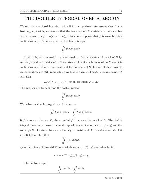
<strong>THE</strong> <strong>DOUBLE</strong> <strong>INTEGRAL</strong> <strong>OVER</strong> A <strong>REGION</strong> 1<br />
<strong>THE</strong> <strong>DOUBLE</strong> <strong>INTEGRAL</strong> <strong>OVER</strong> A <strong>REGION</strong><br />
We start with a closed bounded region Ω in the xy-plane. We assume that Ω is a<br />
basic region; that is, we assume that the boundary of Ω consists of a finite number<br />
of continuous arcs y = φ(x), x = ψ(y). Now let’s suppose that f is some function<br />
continuous on Ω. We want to define the double integral<br />
∫∫<br />
f(x, y) dxdy.<br />
Ω<br />
To do this, we surround Ω by a rectangle R. We now extend f to all of R by<br />
setting f equal to 0 outside of Ω. This extended function f is bounded on R, and it is<br />
continuous on all of R except possibly at the boundary of Ω. In spite of these possible<br />
discontinuities, f is still integrable on R; that is, there still exists a unique number I<br />
such that<br />
L f (P ) ≤ I ≤ U f (P ) for all partitions P of R.<br />
This number I is by definition the double integral<br />
∫∫<br />
R<br />
f(x, y) dxdy.<br />
We define the double integral over Ω by setting<br />
∫∫<br />
Ω<br />
∫∫<br />
f(x, y) dxdy =<br />
R<br />
f(x, y) dxdy.<br />
If f is nonnegative over Ω, the extended f is nonnegative on all of R. The double<br />
integral gives the volume of the solid trapped between the surface z = f(x, y) and the<br />
rectangle R. But since the surface has height 0 outside of Ω, the volume outside of Ω<br />
is 0. It follows then that<br />
∫∫<br />
f(x, y) dxdy<br />
Ω<br />
gives the volume of the solid T bounded above by z = f(x, y) and below by Ω:<br />
volume of T = ∫∫ Ω f(x, y) dxdy.<br />
The double integral<br />
∫∫<br />
∫∫<br />
1 dxdy =<br />
dxdy<br />
Ω<br />
Ω<br />
March 17, 2001
<strong>THE</strong> <strong>DOUBLE</strong> <strong>INTEGRAL</strong> <strong>OVER</strong> A <strong>REGION</strong> 2<br />
gives the volume of a solid of constant height 1 over Ω. In square units this is the area<br />
of Ω:<br />
∫∫<br />
area of Ω = dxdy.<br />
Ω<br />
Below we list four elementary properties of the double integral. They are all analogous<br />
to what was in the one-variable case. The Ω referred to is a basic region. The<br />
functions f and g are assumed to be continuous on Ω.<br />
I. The double integral is linear:<br />
∫∫<br />
Ω<br />
∫∫<br />
[αf(x, y) + βg(x, y)] dxdy = α<br />
II. The double integral preserves order:<br />
Ω<br />
∫∫<br />
f(x, y) dxdy + β g(x, y) dxdy.<br />
Ω<br />
∫∫<br />
if f ≥ 0 on Ω, then<br />
∫∫<br />
if f ≤ g on Ω, then<br />
III. The double integral is additive:<br />
Ω<br />
Ω<br />
f(x, y) dxdy ≥ 0;<br />
∫∫<br />
f(x, y) dxdy ≤ g(x, y) dxdy.<br />
if Ω is broken up into a finite number of basic regions Ω 1 , · · · , Ω n , then<br />
∫∫<br />
∫∫<br />
∫∫<br />
f(x, y) dxdy = f(x, y) dxdy + · · · + f(x, y) dxdy.<br />
Ω<br />
Ω 1<br />
IV. The double integral satisfies a mean-value condition; namely, there is a point<br />
(x 0 , y 0 ) for which<br />
∫∫<br />
Ω<br />
Ω<br />
Ω n<br />
f(x, y) dxdy = f(x 0 , y 0 ) · (the area of Ω).<br />
We call f(x 0 , y 0 ) the average value of f on Ω.<br />
The notion of average given in (IV) enables us to write<br />
∫∫<br />
Ω<br />
f(x, y) dxdy = (the arerage value of f on Ω) · (the area of Ω).<br />
This is a powerful intuitive way of viewing the double integral. We will capitalize on<br />
it as we go on.<br />
March 17, 2001
<strong>THE</strong> EVALUATION OF <strong>DOUBLE</strong> <strong>INTEGRAL</strong>S BY REPEATED <strong>INTEGRAL</strong>S 3<br />
<strong>THE</strong>OREM MEAN-VALUE <strong>THE</strong>OREM FOR <strong>DOUBLE</strong> <strong>INTEGRAL</strong>S.<br />
Let f and g be functions continuous on a basic region Ω. If g is nonnegative on Ω,<br />
then there exists a point (x 0 , y 0 ) in Ω for which<br />
∫∫<br />
∫∫<br />
f(x, y)g(x, y) dxdy = f(x 0 , y 0 ) g(x, y) dxdy.<br />
Ω<br />
We call f(x 0 , y 0 ) the g-weighted average of f on Ω.<br />
Proof. Since f is continuous on Ω and Ω is closed and bounded, we know that f<br />
takes on a minimum value m and a maximum value M. Since g is nonnegative on Ω,<br />
and<br />
Therefore<br />
∫∫<br />
Ω<br />
∫∫<br />
m<br />
mg(x, y)≤ f(x, y)g(x, y) ≤ Mg(x, y)<br />
∫∫<br />
∫∫<br />
mg(x, y) dxdy ≤ f(x, y)g(x, y) dxdy ≤ Mg(x, y) dxdy<br />
Ω<br />
Ω<br />
∫∫<br />
∫∫<br />
g(x, y) dxdy ≤ f(x, y)g(x, y) dxdy ≤ M g(x, y) dxdy.<br />
Ω<br />
We know that ∫∫ Ω g(x, y) dxdy ≥ 0. If ∫∫ Ω g(x, y) dxdy = 0, then from the last<br />
equation we have ∫∫ Ω f(x, y)g(x, y) dxdy = 0 and the theorem holds for all choices of<br />
(x 0 , y 0 ) in Ω. If ∫∫ Ω g(x, y) dxdy > 0, then<br />
∫∫<br />
Ω f(x, y)g(x, y) dxdy<br />
m ≤ ∫∫Ω g(x, y) dxdy ≤ M<br />
and by the intermediate-value theorem there exists (x 0 , y 0 ) in Ω for which<br />
∫∫<br />
Ω f(x, y)g(x, y) dxdy<br />
f(x 0 , y 0 ) = ∫∫Ω g(x, y) dxdy .<br />
Ω<br />
Ω<br />
Ω<br />
Obviously then<br />
∫∫<br />
f(x 0 , y 0 )<br />
∫∫<br />
g(x, y) dxdy =<br />
f(x, y)g(x, y) dxdy.<br />
Ω<br />
Ω<br />
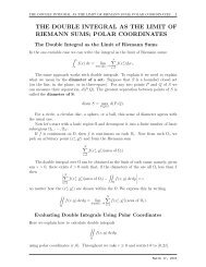
<strong>THE</strong> EVALUATION OF <strong>DOUBLE</strong> <strong>INTEGRAL</strong>S<br />
BY REPEATED <strong>INTEGRAL</strong>S<br />
The Reduction Formulas<br />
If an integral<br />
∫ b<br />
a<br />
f(x) dx<br />
March 17, 2001
<strong>THE</strong> EVALUATION OF <strong>DOUBLE</strong> <strong>INTEGRAL</strong>S BY REPEATED <strong>INTEGRAL</strong>S 4<br />
proves difficult to evaluate, it is not because of the interval [a, b] but because of the<br />
integrand f. Difficulty in evaluating a double integral<br />
∫∫<br />
f(x, y) dxdy<br />
Ω<br />
can come from two sources: from the integrand f and from the base region Ω. Even<br />
such a simple looking integral as ∫∫ Ω 1 dxdy is difficult to evaluate if Ω is complicated.<br />
In this section we introduce a technique for evaluating double integrals of continuous<br />
functions over Ω’s that have a simple structure. The fundamental idea of this section<br />
is that double integrals over sets of this structure can be reduced to a pair of ordinary<br />
integrals.<br />
Type I The projection of Ω onto the x-axis is a closed interval [a, b] and Ω consists<br />
of all points (x, y) with<br />
Then<br />
Here we first calculate<br />
∫∫<br />
Ω<br />
a ≤ x ≤ b and φ 1 (x) ≤ y ≤ φ 2 (x).<br />
f(x, y) dxdy =<br />
∫ φ2 (x)<br />
φ 1 (x)<br />
∫ ( b ∫ φ2 (x)<br />
a<br />
φ 1 (x)<br />
f(x, y) dy<br />
f(x, y) dy<br />
by integrating f(x, y) with respect to y from y = φ 1 (x) to y = φ 2 (x). The resulting<br />
expression is a function of x alone, which we then integrate with respect to x from<br />
x = a to x = b.<br />
Type II. The projection of Ω onto the y-axis is a closed interval [a, b] and Ω consists<br />
of all points (x, y) with<br />
Then<br />
∫∫<br />
This time we first calculate<br />
Ω<br />
a ≤ y ≤ b and φ 1 (y) ≤ x ≤ φ 2 (y).<br />
f(x, y) dxdy =<br />
∫ φ2 (y)<br />
φ 1 (y)<br />
∫ ( b ∫ φ2 (y)<br />
a<br />
φ 1 (y)<br />
f(x, y) dx<br />
f(x, y) dx<br />
by integrating f(x, y) with respect to x from x = φ 1 (y) to x = φ 2 (y). The resulting<br />
expression is a function of y alone, which we then integrate with respect to y from<br />
y = a to y = b. These formulas are easy to understand geometrically.<br />
)<br />
)<br />
dx<br />
dy.<br />
The Reduction Formulas March 17, 2001
Computations 5<br />
The Reduction Formulas Viewed Geometrically<br />
Let’s take f as nonnegative and Ω of type I. The double integral over Ω gives the<br />
volume of the solid T that is trapped between Ω and the surface z = f(x, y) :<br />
∫∫<br />
Ω<br />
f(x, y) dxdy = volume of T.<br />
We can also compute the volume of T by the method of parallel cross sections. Let<br />
A(x) be the area of that cross section of T that has first coordinate x. Then<br />
∫ b<br />
Since<br />
A(x) =<br />
we have<br />
a<br />
∫ ( b ∫ φ2 (x)<br />
a φ 1 (x)<br />
A(x)dx = volume of T.<br />
∫ φ2 (x)<br />
φ 1 (x)<br />
f(x, y) dy<br />
)<br />
f(x, y) dy,<br />
dx = volume of T.<br />
Combining the two equations, we have the first reduction formula<br />
∫∫<br />
∫ ( b ∫ )<br />
φ2 (x)<br />
f(x, y) dxdy =<br />
f(x, y) dy dx.<br />
a φ 1 (x)<br />
Ω<br />
The other reduction formula can be obtained in a similar manner.<br />
Computations<br />
Problem 1. Evaluate<br />
with Ω the region bounded by<br />
∫∫<br />
Ω<br />
(x 2 − y) dxdy<br />
y = x 2 , y = −x 2 , x = −1, x = 1.<br />
Solution. By projecting Ω onto the x-axis we obtain the interval [−1, 1]. The region Ω<br />
consists of all points (x, y) with<br />
−1 ≤ x ≤ 1 and − x 2 ≤ y ≤ x 2 .<br />
March 17, 2001
Computations 6<br />
This is a region of type I.<br />
∫∫<br />
∫ 1<br />
( ∫ x 2<br />
)<br />
(x 2 − y) dxdy = (x 2 − y) dy dx<br />
−1 −x 2<br />
Ω<br />
=<br />
∫ 1<br />
−1<br />
[x 2 y − 1 2 y2 ] x 2<br />
Problem 2. Evaluate<br />
with Ω bounded by<br />
=<br />
−x 2 dx =<br />
∫ 1<br />
−1<br />
∫ 1<br />
−1<br />
[<br />
(x 4 − 1 2 x4 ) − (−x 4 − 1 ]<br />
2 x4 ) dx<br />
[ ] 2 1<br />
2x 4 dx =<br />
5 x5 = 4<br />
−1 5 .<br />
∫∫<br />
(xy − y 3 ) dxdy<br />
Ω<br />
y = 0, x = y, y = 1, x = −1.<br />
Solution. By projecting Ω onto the y-axis we obtain the interval [0, 1]. The region<br />
Ω consists of all points (x, y) with<br />
This is a region of type II.<br />
=<br />
0 ≤ y ≤ 1 and −1 ≤ x ≤ y.<br />
∫∫<br />
∫ 1 (∫ y<br />
)<br />
(xy − y 3 ) dxdy = (xy − y 3 ) dx dy<br />
0 −1<br />
Ω<br />
∫ 1 [ ] 1 y ∫ 1<br />
0 2 x2 y − xy 3 dy = (− 1<br />
−1 0 2 y − 1 2 y3 − y 4 )dy<br />
[ 1<br />
=<br />
4 y2 − 1 8 y4 − 1 ] 1<br />
5 y5 0<br />
= − 23<br />
40 .<br />
We can also project Ω onto the x-axis and express Ω as a region of type I, but<br />
then the lower boundary is defined piecewise and the calculations are somewhat more<br />
complicated: setting<br />
φ(x) =<br />
we have Ω as the set of all points (x, y) with<br />
⎧<br />
⎪ ⎨<br />
⎪ ⎩<br />
0, if − 1 ≤ x ≤ 0<br />
x if 0 ≤ x ≤ 1<br />
−1 ≤ x ≤ 1 and φ(x) ≤ y ≤ 1;<br />
,<br />
thus<br />
∫∫<br />
Ω<br />
∫ ( 1 ∫ )<br />
1<br />
(xy − y 3 ) dxdy = (xy − y 3 ) dy dx<br />
−1 φ(x)<br />
March 17, 2001
Computations 7<br />
=<br />
∫ 0<br />
=<br />
−1<br />
∫ 0<br />
( ∫ 1<br />
−1<br />
Repeated integrals<br />
)<br />
(xy − y 3 ) dy<br />
φ(x)<br />
(∫ 1<br />
)<br />
(xy − y 3 ) dy<br />
0<br />
∫ ( b ∫ φ2 (x)<br />
a<br />
φ 1 (x)<br />
dx +<br />
dx +<br />
∫ ( 1 ∫ 1<br />
0<br />
∫ 1 (∫ 1<br />
= (− 1 2 ) + (− 3 40 ) = −23 40 .<br />
f(x, y) dy<br />
)<br />
dx and<br />
0<br />
(xy − y 3 ) dy<br />
φ(x)<br />
)<br />
x<br />
∫ ( b ∫ φ2 (y)<br />
a<br />
(xy − y 3 ) dy<br />
φ 1 (y)<br />
f(x, y) dx<br />
can be written in more compact form by omitting the large parentheses. From now on<br />
we will simply write<br />
)<br />
)<br />
dx<br />
dx<br />
dy<br />
∫ b ∫ φ2 (x)<br />
a φ 1 (x)<br />
f(x, y) dydx and<br />
∫ b ∫ φ2 (y)<br />
a φ 1 (y)<br />
f(x, y) dxdy.<br />
Problem 3. Evaluate<br />
with Ω the region bounded by<br />
∫∫<br />
Ω<br />
(x 1/2 − y 2 ) dxdy<br />
y = x 2 and x = y 4 .<br />
Solution. The projection of Ω onto the x-axis is the closed interval [0, 1], and Ω can<br />
be characterized as the set of all (x, y) with<br />
0 ≤ x ≤ 1 and x 2 ≤ y ≤ x 1/4 .<br />
Thus<br />
∫∫<br />
∫ 1 ∫ x 1/4<br />
(x 1/2 − y 2 ) dxdy = (x 1/2 − y 2 ) dydx<br />
0 x 2<br />
Ω<br />
∫ 1<br />
=<br />
[x 1/2 y − 1 ] x 1/4 ∫ 1<br />
0 3 y3 dx = ( 2<br />
x 2 0 3 x3/4 − x 5/2 + 1 3 x6 ) dx<br />
[ 8<br />
=<br />
21 x7/4 − 2 7 x7/2 + 1 ] 1<br />
21 x7 = 1<br />
0 7 .<br />
We can also integrate in the other order. The projection of Ω onto the y-axis is the<br />
closed interval [0, l], and Ω can be characterized as the set of all (x, y) with<br />
0 ≤ y ≤ 1 and y 4 ≤ x ≤ y 1/2 .<br />
March 17, 2001
Computations 8<br />
This gives the same result:<br />
∫∫<br />
∫ 1 ∫ y 1/2<br />
(x 1/2 − y 2 ) dxdy = (x 1/2 − y 2 ) dxdy<br />
0 y 4<br />
Ω<br />
=<br />
∫ 1<br />
0<br />
( 2 3 y3/4 − y 5/2 + 1 3 y6 )dy = 1 7 .<br />
Problem 4. Calculate by double integration the area of the region Ω that lies<br />
between<br />
√ √ √ x + y = a and x + y = a.<br />
Solution. The area of Ω is given by the double integral<br />
∫∫<br />
Ω<br />
dxdy.<br />
Here again we can integrate in either order. We can project Ω onto the x- axis and<br />
write the boundaries as functions of x:<br />
Ω is then the set of all (x, y) with<br />
This gives<br />
y = ( √ a − √ x) 2 and y = a − x;<br />
0 ≤ x ≤ a and ( √ a − √ x) 2 ≤ y ≤ a − x.<br />
∫∫<br />
Ω<br />
∫ a<br />
=<br />
0<br />
dxdy =<br />
∫ a ∫ a−x<br />
0<br />
( √ a− √ x) 2 dydx<br />
(−2x + 2 √ a √ x) dx = a2<br />
3 .<br />
We can also project Ω onto the y-axis and write the boundaries as functions of y:<br />
Ω is then the set of all (x, y) with<br />
x = ( √ a − √ y) 2 and x = a − y;<br />
0 ≤ y ≤ a and ( √ a − √ y) 2 ≤ x ≤ a − y.<br />
This gives<br />
∫∫<br />
Ω<br />
dxdy =<br />
∫ a ∫ a−y<br />
0<br />
( √ a− √ y) 2 dxdy,<br />
which is also a2<br />
3 . March 17, 2001
Symmetry in Double Integration 9<br />
Symmetry in Double Integration<br />
First we go back to the one-variable case. Let’s suppose that g is continuous on an<br />
interval that is symmetric about the origin, say [−a, a].<br />
If g is odd, then ∫ a<br />
−a g(x)dx = 0.<br />
If g is even, then ∫ a<br />
−a g(x)dx = 2 ∫ a<br />
0 g(x)dx.<br />
We have similar results for double integrals.<br />
Suppose that Ω is symmetric about the y-axis.<br />
If f is odd in x [if f(−x, y) = −f(x, y)], then ∫∫ Ω f(x, y) dxdy = 0.<br />
If f is even in x [if f(−x, y) = f(x, y)], then<br />
∫∫<br />
Ω f(x, y) dxdy = 2 ∫∫ right half of Ω f(x, y) dxdy.<br />
Suppose that Ω is symmetric about the x-axis.<br />
If f is odd in y [if f(x, −y) = −f(x, y)], then ∫∫ Ω f(x, y) dxdy = 0.<br />
If f is even in y [if f(x, −y) = f(x, y)], then<br />
∫∫<br />
Ω f(x, y) dxdy = 2 ∫∫ upper half of Ω f(x, y) dxdy.<br />
As an example take the region bounded by<br />
x + y = 0, x − y = 0, x = a, x = −a.<br />
Suppose we wanted to calculate<br />
∫∫<br />
Ω<br />
(2x − sin x 2 y) dxdy.<br />
Symmetry about the y-axis gives<br />
∫∫<br />
2x dxdy = 0.(integrand is odd in x)<br />
Ω<br />
Symmetry about the x-axis gives<br />
∫∫<br />
sin x 2 y dxdy = 0.(integrand is odd in y)<br />
Ω<br />
March 17, 2001
Symmetry in Double Integration 10<br />
Therefore<br />
∫∫<br />
(2x − sin x 2 y) dxdy = 0.<br />
Ω<br />
As another example we go to Problem 1 and reevaluate<br />
∫∫<br />
Ω<br />
(x 2 − y) dxdy,<br />
this time capitalizing on the symmetry of Ω. Note that<br />
Therefore<br />
∫∫<br />
Ω<br />
∫∫<br />
Ω<br />
x 2 dxdy = 2<br />
ydxdy = 0 (symmetric about x − axis)<br />
∫∫<br />
right half of Ω<br />
= 4<br />
x 2 dxdy = 0 (symmetric about y − axis)<br />
∫∫<br />
upper part<br />
of the right half of Ω<br />
x 2 dxdy.<br />
∫∫<br />
∫ 1 ∫ x 2<br />
(x 2 − y) dxdy = 4 x 2 dydx = 4<br />
0 0<br />
5 .<br />
Ω<br />
Problem 5. Calculate the volume within the cylinder<br />
x 2 + y 2 = b 2<br />
between the planes<br />
y + z = a 2<br />
and<br />
z = 0<br />
given that<br />
a 2 ≥ b > 0.<br />
Solution. The solid in question is bounded below by the disc<br />
Ω : 0 ≤ x 2 + y 2 ≤ b 2<br />
and above by the plane<br />
z = a 2 − y.<br />
March 17, 2001
Concluding Remarks 11<br />
The volume is given by the double integral<br />
Since Ω is symmetric about the x-axis,<br />
Thus<br />
Ω<br />
∫∫<br />
(a 2 − y) dxdy.<br />
Ω<br />
∫∫<br />
Ω<br />
Ω<br />
y dxdy = 0.<br />
∫∫<br />
∫∫<br />
(a 2 − y) dxdy = a 2 dxdy = a 2 (area of Ω) = πa 2 b 2 .<br />
Concluding Remarks<br />
When two orders of integration are possible, one order may be easy to carry out, while<br />
the other may present serious difficulties. Take as an example the double integral<br />
with Ω bounded by<br />
Projection onto the x-axis leads to<br />
Projection onto the y-axis leads to<br />
∫∫<br />
Ω<br />
cos 1 2 πx2 dxdy<br />
y = x, y = 0, x = 1.<br />
∫ 1 ∫ x<br />
0<br />
0<br />
∫ 1 ∫ 1<br />
0<br />
y<br />
cos 1 2 πx2 dydx.<br />
cos 1 2 πx2 dxdy.<br />
The first expression is easy to calculate, but the second is not. The only practical way<br />
to handle the second expression is to expand cos 1 πx as a series in x and then integrate<br />
2<br />
term by term.<br />
Finally, if Ω, the region of integration, is neither of type I nor of type II, it is usually<br />
possible to break it up into a finite number of regions Ω 1 , · · · , Ω n , each of type I or type<br />
II. Since the double integral is additive,<br />
∫∫<br />
Ω 1<br />
∫∫<br />
Ω n<br />
∫∫<br />
Ω<br />
f(x, y) dxdy + · · · + f(x, y) dxdy = f(x, y) dxdy.<br />
Each of the integrals on the left can be evaluated by the methods of this section.<br />
March 17, 2001
Exercise 12<br />
Exercise<br />
1. Evaluate the integrals<br />
(a) ∫ 3 ∫ 2<br />
0 0 (4 − y2 )dydx [16]<br />
(b) ∫ 0 ∫ 1<br />
−1 −1 (x + y + 1)dxdy [1]<br />
(c) ∫ π<br />
0<br />
(d) ∫ ln 8<br />
1<br />
∫ x<br />
0 x sin ydydx [2 + 1 2 π2 ]<br />
∫ ln y<br />
0 e x+y dxdy [24 ln 2 − 16 + e]<br />
(e) ∫ 1 ∫ y 2<br />
0 0 3y 3 e xy dxdy [e − 2]<br />
(f) ∫ 0 ∫ −v<br />
−2 v 2dpdv [8]<br />
(g) ∫ π/3 ∫ sec t<br />
−π/3 0 3 cos tdudt [2π]<br />
(h) ∫ π<br />
0<br />
∫ π<br />
x<br />
(i) ∫ 2 √ ln 3<br />
0<br />
sin y<br />
y<br />
dydx [2]<br />
∫ √ ln 3<br />
y/2 e x2 dxdy [2]<br />
(j) ∫ 3 ∫<br />
√ 1<br />
0 x/3 ey2 dydx [e − 1]<br />
2. Write an equivalent double integral with the order of integration reversed.<br />
(a) ∫ 1 ∫ 4−2x<br />
0 2 dydx [ ∫ 4 ∫ (4−y)/2<br />
2 0 dxdy]<br />
(b) ∫ 1 ∫ √ y<br />
0 y dxdy [ ∫ 1 ∫ x<br />
0 x dydx]<br />
2<br />
(c) ∫ 1 ∫ e x<br />
0 0 dydx [ ∫ e ∫ 1<br />
1 ln y dxdy]<br />
(d) ∫ 3/2<br />
0<br />
(e) ∫ 1<br />
0<br />
∫ 9−4x 2<br />
0 dydx [ ∫ 9<br />
0<br />
∫ √ ( 9−y)/2<br />
0 dxdy]<br />
∫ √ 1−y 2<br />
−<br />
√1−y dxdy [∫ 1 ∫ √ 1−x 2<br />
2 −1 0 dydx]<br />
3. Find the volume of the solid whose base is the region in the xy-plane that is<br />
bounded by the parabola y = 4 − x 2 and the line y = 3x, while the top of the<br />
solid is bounded by the plane z = x + 4. [ 625<br />
12 ]<br />
4. Find the volume of the solid in the first octant bounded by the coordinate planes,<br />
the plane x = 3, and the parabolic cylinder z = 4 − y 2 . [16]<br />
5. Find the volume of the region that lies under the paraboloid z = x 2 + y 2 and<br />
above the triangle enclosed by the lines y = x, x = 0, and x + y = 2 on the<br />
xy-plane. [4/3]<br />
March 17, 2001