Mean-Value Theorem (Several Variables)

Mean-Value Theorem (Several Variables) 1
Mean-Value Theorem (Several Variables)
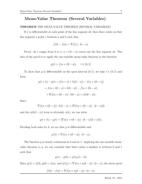
THEOREM THE MEAN-VALUE THEOREM (SEVERAL VARIABLES)
If f is differentiable at each point of the line segment ab, then there exists on that
line segment a point c between a and b such that
f(b) − f(a) = ∇f(c) · (b − a).
Proof. As t ranges from 0 to 1, a + t(b − a) traces out the line segment ab. The
idea of the proof is to apply the one-variable mean-value theorem to the function
g(t) = f(a + t[b − a]), t ∈ [0, 1].
To show that g is differentiable on the open interval (0, 1), we take t ∈ (0, 1) and
form
g(t + h) − g(t) = f(a + (t + h)[b − a]) − f(a + t[b − a])
= f(a + t[b − a] + h[b − a]) − f(a + t[b − a])
= ∇f(a + t[b − a]) · h[b − a] + o(h[b − a]).
Since
∇f(a + t[b − a]) · h(b − a) = [∇f(a + t[b − a]) · (b − a)]h
and the o(h(b − a)) term is obviously o(h), we can write
g(t + h) − g(t) = [∇f(a + t[b − a]) · (b − a)]h + o(h).
Dividing both sides by h, we see that g is differentiable and
g ′ (t) = ∇f(a + t[b − a]) · (b − a).
The function g is clearly continuous at 0 and at 1. Applying the one-variable meanvalue
theorem to g, we can conclude that there exists a number t 0 between 0 and 1
such that
g(1) − g(0) = g ′ (t 0 )(1 − 0).
Since g(1) = f(b), g(0) = f(a), and g ′ (t 0 ) = ∇f(a + t 0 [b − a]) · (b − a), the above gives
f(b) − f(a) = ∇f(a + t 0 [b − a]) · (b − a).
March 17, 2001

Mean-Value Theorem (Several Variables) 2
Setting c = a + t 0 [b − a], we have
f(b) − f(a) = ∇f(c) · (b − a).
A nonempty open set U (in the plane or in three-space) is said to be connected if
any two points of U can be joined by a polygonal path that lies entirely in U.
THEOREM. Let U be an open connected set. If ∇f(x) = 0 for all x ∈ U, then f
is constant in U.
Proof. Let a and b be any two points in U. Since U is open and connected, we can
join these points by a polygonal path with vertices a = c 0 , c 1 , · · · , c n−1 , c n = b. By the
mean-value theorem there exist points
c ∗ 1 on c 0 c 1 such that f(c 1 ) − f(c 0 ) = ∇f(c1) ∗ · (c 1 − c 0 ),
c ∗ 2 on c 1 c 2 such that f(c 2 ) − f(c 1 ) = ∇f(c2) ∗ · (c 2 − c 1 ),
c ∗ 3 on c 2 c 3 such that f(c 3 ) − f(c 2 ) = ∇f(c3) ∗ · (c 3 − c 2 ),
· · ·
c ∗ n on c n−1 c n such that f(c n ) − f(c n−1 ) = ∇f(cn) ∗ · (c n − c n−1 ).
If ∇f(x) = 0 for all x in U, then
f(c 1 ) − f(c 0 ) = 0, f(c 2 ) − f(c 1 ) = 0, · · · , f(c n ) − f(c n−1 ) = 0
This shows that
f(a) = f(c 0 ) = f(c 1 ) = f(c 2 ) = · · · = f(c n−1 ) = f(c n ) = f(b).
Since a and b are arbitrary points of U, f must be constant on U.
THEOREM. Let U be an open connected set.
If ∇f(x) = ∇g(x) for all x in U, then f and g differ by a constant on U.
Proof. If ∇f(x) = ∇g(x) for all x in U, then
∇[f(x) − g(x)] = ∇f(x) − ∇g(x) = 0
for all x in U. Therefore, f − g must be constant on U.
March 17, 2001

Continuity on a Closed Region 3
We have seen that a function continuous on an interval skips no values. (The
intermediate-value theorem .) There are analogous results for functions of several
variables. Here is one of them.
THEOREM AN INTERMEDIATE-VALUE THEOREM (SEVERAL VARIABLES)
Suppose that f is continuous on an open connected set U and A < C < B. If,
somewhere on U, f takes on the value A and, somewhere on U, f takes on the value
B, then, somewhere on U, f takes on the value C.
Proof. Let a and b be points of U for which
f(a) = A and f(b) = B.
We must show that there exists a point c in U for which f(c) = C.
Since U is polygonally connected, there is a polygonal path in U
r = r(t), t ∈ [a, b]
that joins a to b. Since r is continuous on [a, b], the composition
g(t) = f(r(t))
is also continuous on [a, b]. Since
g(a) = f(r(a)) = f(a) = A and g(b) = f(r(b)) = f(b) = B,
we know from the intermediate-value theorem of one variable that there is a number c
in [a, b] for which g(t) = C. Setting c = r(t) we have f(c) = C.
Continuity on a Closed Region
An open connected set is called an open region. If we start with an open region and
adjoin to it the boundary, then we have what is called a closed region. (A closed
region is therefore a closed set, the interior of which is an open region.)
Continuity on a closed region Ω requires continuity at the boundary points of Ω as
well as the interior points.
If x 0 is an interior point of Ω, then all points x sufficiently close to x 0 are in Ω and,
by definition, f is continuous at x 0 if as x approaches x 0 , f(x) approaches f(x 0 ).
March 17, 2001

Continuity on a Closed Region 4
If x 0 is a boundary point of Ω, then we have to modify the definition and say: f is
continuous at x 0 if as x approaches x 0 within Ω, f(x) approaches f(x 0 ).
In terms of ɛ − δ, f is continuous at a boundary point x 0 if for each ɛ > 0 there
exists δ> 0 such that
if ‖x − x 0 ‖ < δ and x ∈ Ω, then |f(x) − f(x 0 )| < ɛ.
(This is completely analogous to one-sided continuity at an endpoint of a closed
interval [a, b].)
The intermediate-value result that we just proved for open connected sets can be
extended to closed regions.
THEOREM A SECOND INTERMEDIATE-VALUE THEOREM [SEVERAL VARI-
ABLES]
Suppose that f is continuous on a closed region Ω and A < C < B. If, somewhere
on Ω, f takes on the value A and, somewhere on Ω, f takes on the value B, then,
somewhere on Ω, f takes on the value C.
Proof. Let a and b be points of Ω for which
f(a) = A and f(b) = B.
If a and b are both in the interior of Ω, then the result follows from the previous
theorem. But one or both of these points could lie on the boundary of Ω. To take care
of that possibility, we can proceed as follows. Take ɛ > 0 small enough that
A + ɛ < C < B − ɛ.
By continuity there exist points x 1 , x 2 in the interior of Ω for which
f(x 1 ) < A + ɛ and B − ɛ < f(x 2 ).
Then
f(x 1 ) < C < f(x 2 )
and the result follows from the previous theorem.
March 17, 2001

Chain Rules 5
Chain Rules
For functions of a single variable there is basically only one chain rule. For functions
of several variables there are many chain rules.
A vector-valued function is said to be continuous provided that its components are
continuous. If f = f(x, y, z) is a scalar-valued function (a real-valued function), then
its gradient ∇f is a vector-valued function. We say that f is continuously differentiable
on an open set U if f is differentiable on U and ∇f is continuous on U. If a curve r
lies in the domain of f then we can form the composition
(f ◦ r)(t) = f(r(t)).
The composition f ◦r is a real-valued function of a real variable t. The numbers f(r(t))
are the values taken on by f along the curve r.
THEOREM CHAIN RULE (ALONG A CURVE)
If f is continuously differentiable on an open set U and r = r(t) is a differentiable
curve that lies entirely in U, then the composition f ◦ r is differentiable and
Proof. We will show that
d
dt [(f ◦ r)(t)] = ∇f(r(t)) · r′ (t).
f(r(t + h)) − f(r(t))
lim
h→0 h
= ∇f(r(t)) · r ′ (t).
For h ≠ 0 and sufficiently small, the line segment that joins r(t) to r(t + h) lies entirely
in U. This we know because U is open and r is continuous. For such h, the meanvalue
theorem we just proved assures us that there exists a point c(h) between r(t) and
r(t + h) such that
Dividing both sides by h, we have
f(r(t + h)) − f(r(t)) = ∇f(c(h)) · [r(t + h) − r(t)].
f(r(t + h)) − f(r(t))
h
= ∇f(c(h)) · [
r(t + h) − r(t)
].
h
As h tends to zero, c(h) tends to r(t) and by the continuity of ∇f,
∇f(c(h)) → ∇f(r(t)).
March 17, 2001

Chain Rules 6
Since
the result follows.
r(t + h) − r(t)
h
→ r ′ (t),
Problem 1. Use the chain rule to find the rate of change of
f(x, y) = 1 3 (x3 + y 3 )
with respect to t along the curve r(t) = a cos t i + b sin t j.
Solution. The rate of change of f with respect to t along the curve r is the derivative
d
dt [f(r(t)].
By the chain rule
Here
d
dt [f(r(t)] = ∇f(r(t)) · r′ (t).
∇f = x 2 i + y 2 j.
With x(t) = a cos t and y(t) = b sin t, we have
∇f(r(t)) = a 2 cos 2 t i + b 2 sin 2 t j.
Since r ′ (t) = −a sin t i + b cos t j, we see that
d
dt [f(r(t)] = ∇f(r(t)) · r′ (t)
= (a 2 cos 2 t i + b 2 sin 2 t j) · (−a sin t i + b cos t j)
= −a 3 sin t cos 2 t + b 3 sin 2 t cos t
= sin t cos t (b 3 sin t − a 3 cos t).
Remark. Note that we could have obtained the same result without invoking the
chain rule by first forming f(r(t)) and then differentiating:
f(r(t)) = f(x(t), y(t)) = 1 3 ([x(t)]3 + [y(y)] 3 ) = 1 3 (a3 cos 3 t + b 3 sin 3 t)
so that
d
dt [f(r(t))] = 1 3 [3a3 cos 2 t(− sin t) + 3b 3 sin 2 t cos t]
March 17, 2001

Another Formulation of the Chain Rule 7
= sin t cos t (b 3 sin t − a 3 cos t).
Problem 2. Use the chain rule to find the rate of change of
f(x, y, z) = x 2 y + z cos x
with respect to t along the twisted cubic r(t) = ti + t 2 j + t 3 k.
Solution. Once again we use the relation
d
dt [f(r(t)] = ∇f(r(t)) · r′ (t).
This time
∇f = (2xy − z sin x, x 2 , cos x).
With x(t) = t, y(t) = t 2 , z(t) = t 3 , we have
∇f(r(t)) = (2t 3 − t 3 sin t, t 2 , cos t).
Since r ′ (t) = (1, 2t, 3t 2 ), we have
d
dt [f(r(t)] = ∇f(r(t)) · r′ (t).
= (2t 3 − t 3 sin t, t 2 , cos t) · (1, 2t, 3t 2 )
= 2t 3 − t 3 sin t + 2t 3 + 3t 2 cos t
= 4t 3 − t 3 sin t + 3t 2 cos t.
Another Formulation of the Chain Rule
The chain rule for functions of one variable,
d
dt [u(x(t))] = u′ (x(t))x ′ (t),
can be written
In a similar manner, the relation
du
dt = du dx
dx dt .
d
dt [f(r(t)] = ∇f(r(t)) · r′ (t)
March 17, 2001

Another Formulation of the Chain Rule 8
can be written
With
this equation takes the form
∇u = ( ∂u
∂x , ∂u
du
dt
∂y , ∂u
∂z
= ∇u · dr
dt .
) and
dr
dt = (dx dt , dy
dt , dz
dt ),
du
dt = ∂u dx
∂x dt + ∂u dy
∂y dt + ∂u dz
∂z dt .
In the two-variable case, the z-term drops out and we have
Problem 3. Find du/dt if
du
dt = ∂u dx
∂x dt + ∂u dy
∂y dt .
u = x 2 − y 2 and x = t 2 − 1, y = 3 sin πt.
Solution. Here we are in the two-variable case
du
dt = ∂u dx
∂x dt + ∂u dy
∂y dt .
Since
we have
∂u
∂x
= 2x,
∂u
∂y
du
dt
= −2y and
dx
dt
= 2t,
dy
dt
= (2x)(2t) + (−2y)(3π cos πt)
= 4t 3 − 4t − 18π sin πt cos πt.
= 3π cos πt,
This same result may be obtained by first writing u directly as a function of t and
then differentiating:
so that
u = x 2 − y 2 = (t − 1) 2 − (3 sin πt) 2
du
dt = 4t3 − 4t − 18π sin πt cos πt.
Problem 4. The upper radius of the frustum of a cone is 10 inches, the lower
radius is 12 inches, and the height is 18 inches. At what rate is the volume changing if
the upper radius decreases at the rate of 2 inches per minute, the lower radius increases
March 17, 2001

Other Chain Rules 9
at the rate of 3 inches per minute, and the height decreases at the rate of 4 inches per
minute
Solution. Let x be the upper radius, y the lower radius, and z the height. Then
V = 1 3 πz(x2 + xy + y 2 )
so that
∂V
∂x = 1 ∂V
πz(2x + y),
3 ∂y = 1 ∂V
πz(x + 2y),
3 ∂z = 1 3 π(x2 + xy + y 2 ).
Since
we have here
dV
dt = ∂V dx
∂x dt + ∂V dy
∂y dt + ∂V
∂z
dz
dt ,
Set
we find that
dV
dt = 1 πz(2x + y)dx
3 dt + 1 πz(x + 2y)dy
3 dt + 1 3 π(x2 + xy + y 2 ) dz
dt .
x = 10, y = 12, z = 18, dx
dt
= −2,
dy
dt
dV
dt = −772 3 π.
= 4,
dz
dt = −4
The volume decreases at the rate of 772/3 cubic inches per minute.
Other Chain Rules
In the setting of functions of several variables there are numerous chain rules. They
can all be deduced from the theorem proved above and its corollaries. If, for example,
u = u(x, y), where x = x(s, t) and y = y(s, t),
then
∂u
∂s = ∂u ∂x
∂x ∂s + ∂u ∂y
∂y ∂s
∂u
and
∂t = ∂u ∂x
∂x ∂t + ∂u
∂y
To obtain the first equation, keep t fixed and differentiate u with respect to s according
to the formula in the chain rule; to obtain the second equation, keep s fixed and
differentiate u with respect to t.
∂y
∂t .
March 17, 2001

Other Chain Rules 10
In the figure below we have drawn a tree diagram for the formula. We construct
such a tree by branching at each stage from a function to all the variables that directly
determine it. Each path starting at u and ending at a variable determines a product
of (partial) derivatives. The partial derivative of u with respect to each variable is the
sum of the products generated by all the direct paths to that variable.
Suppose, for example, that
u = u(x, y, z), where x = x(s, t), y = y(s, t), z = z(s, t).
The partials of u with respect to s and t can be read from the diagram:
∂u
∂s = ∂u ∂x
∂x ∂s + ∂u ∂y
∂y ∂s + ∂u ∂z
∂z ∂s
∂u
and
∂t = ∂u ∂x
∂x ∂t + ∂u ∂y
∂y ∂t + ∂u
∂z
Problem 5. (Implicit differentiation) Let u = u(x, y, z) be a continuously differentiable
function, and suppose that the equation
u(x, y, z) = 0
defines z implicitly as a differentiable function of x and y. Show that
if ∂u
∂z
∂z
≠ 0, then
∂x = −∂u/∂x ∂u/∂z
Solution. To be able to apply the chain rule, we write
Then
Since u(s, t, z(s, t)) = 0 for all s and t,
and
∂z
∂y = −∂u/∂y ∂u/∂z .
u = u(x, y, z) with x = s, y = t, z = z(s, t).
∂u
∂s = ∂u ∂x
∂x ∂s + ∂u ∂y
∂y ∂s + ∂u ∂z
∂z ∂s .
∂z
∂t .
∂u
∂s = 0. March 17, 2001

A first-order partial differential equation with constant coefficients 11
Since
we have
If ∂u
∂z
≠ 0, then
∂z
The formula for ∂z
∂y
0 = ∂u
∂x · 1 + ∂u
∂x
∂s
∂y · 0 + ∂u
∂z
= 1 and
∂y
∂s = 0,
∂z
∂s = ∂u
∂x + ∂u
∂z
∂x = −∂u/∂x ∂u/∂z
can be obtained in a similar manner.
∂z
∂s = ∂u
∂x + ∂u ∂z
∂z ∂x .
A first-order partial differential equation with constant
coefficients
Consider the first-order partial differential equation
∂f(x, y) ∂f(x, y)
3 + 2
∂x ∂y
All the solutions of this equation can be found by geometric considerations. We express
= 0.
the left member as a dot product, and write the equation in the form
(3, 2) · ∇f(x, y) = 0.
This tells us that the gradient vector ∇f(x, y) is orthogonal to the vector 3i + 2j at
each point (x, y). But we also know that ∇f(x, y) is orthogonal to the level curves of
f. Hence these level curves must be straight lines parallel to 3i + 2j. In other words,
the level curves of f are the lines
2x − 3y = c.
Therefore f(x, y) is constant when 2x − 3y is constant. This suggests that
f(x, y) = g(2x − 3y)
for some function g.
March 17, 2001

A first-order partial differential equation with constant coefficients 12
Now we verify that, for each differentiable function g, the scalar field f defined by
this equation does, indeed, satisfy the given PDE. Using the chain rule to compute the
partial derivatives of f we find
∂f
∂x = 2g′ (2x − 3y),
∂f
∂y = −3g′ (2x − 3y),
3 ∂f
∂x + 2∂f ∂y = 6g′ (2x − 3y) − 6g ′ (2x − 3y) = 0.
Therefore, f satisfies the PDE as required.
Conversely, we can show that every differentiable f which satisfies the PDE must
necessarily have the form
f(x, y) = g(2x − 3y)
for some g. To do this, we introduce a linear change of variables,
x = Au + Bv,
y = Cu + Dv.
This transforms f(x, y) into a function of u and v, say
h(u, v) = f(Au + Bv, Cu + Dv).
We shall choose the constants A, B, C, D so that h satisfies the simpler equation
∂h(u, v)
∂u
= 0.
Then we shall solve this equation and show that f has the required form. Using the
chain rule we find
Since f satisfies
∂h
∂u = ∂f ∂x
∂x ∂u + ∂f ∂y
∂y ∂u = ∂f
∂x A + ∂f
∂y C.
∂f(x, y) ∂f(x, y)
3 + 2
∂x ∂y
= 0.
we have ∂f/∂y = −(3/2)(∂f/∂x), so the equation for ∂h/∂u becomes
Therefore, h will satisfy ∂h(u,v)
∂u
find
∂h
∂u = ∂f
∂x (A − 3 2 C).
= 0 if we choose A = 3 C. Taking A = 3 and C = 2 we
2
x = 3u + Bv,
y = 2u + Dv.
March 17, 2001

A first-order partial differential equation with constant coefficients 13
For this choice of A and C, the function h satisfies ∂h(u,v)
∂u
of v alone, say
h(u, v) = g(v)
= 0, so h(u, v) is a function
for some function g. To express v in terms of x and y we eliminate u from
x = 3u + Bv,
y = 2u + Dv
and obtain 2x − 3y = (2B − 3D)v. Now we choose B and D to make 2B − 3D = 1,
say B = 2, D = 1. For this choice the transformation
x = Ax + Bv,
y = Cu + Dv.
is nonsingular; we have v = 2x − 3y, and hence
f(x, y) = h(u, v) = g(v) = g(2x − 3y).
This shows that every differentiable solution for
has the form
∂f(x, y) ∂f(x, y)
3 + 2
∂x ∂y
f(x, y) = g(2x − 3y).
Exactly the same type of argument proves the following theorem for first-order
equations with constant coefficients.
THEOREM Let g be differentiable on R, and let f be the scalar field defined on
R 2 by the equation
f(x, y) = g(bx − ay),
where a and b are constants, not both zero.
differential equation
∂f(x, y) ∂f(x, y)
a + b
∂x ∂y
= 0
Then f satisfies the first-order partial
everywhere in R 2 . Conversely, every differentiable solution of this PDE necessarily
has the form for some g.
= 0
March 17, 2001

d’Alembert’s Solution of the Wave Equation 14
The one-dimensional wave equation
Imagine a string of infinite length stretched along the x-axis and allowed to vibrate
in the xy-plane. We denote by y = f(x, t) the vertical displacement of the string at
the point x at time t. We assume that, at time t = 0, the string is displaced along a
prescribed curve, y = F (x). We regard the displacement f(x, t) as an unknown function
of x and t to be determined. A mathematical model for this problem (suggested by
physical considerations) is the partial differential equation
∂ 2 f
∂t 2
= c2 ∂2 f
∂x 2 ,
where c is a positive constant depending on the physical characteristics of the string.
This equation is called the one-dimensional wave equation. We will solve this
equation subject to certain auxiliary conditions.
Since the initial displacement is the prescribed curve y = F (x), we seek a solution
satisfying the condition
f(x, 0) = F (x).
We also assume that ∂y/∂t, the velocity of the vertical displacement, is prescribed at
time t = 0, say
D 2 f(x, 0) = G(x),
where G is a given function. It seems reasonable to expect that this information
should suffice to determine the subsequent motion of the string. We will show that,
indeed, this is true by determining the function f in terms of F and G. The solution is
expressed in a form given by Jean d’Alembert (1717˜ 1783), a French mathematician
and philosopher.
d’Alembert’s Solution of the Wave Equation
Theorem. Let F and G be given functions such that G is differentiable and F is twice
differentiable on R. Then the function f given by the formula
f(x, t) =
F (x + ct) + F (x − ct)
2
+ 1 2c
∫ x+ct
x−ct
G(s) ds
March 17, 2001

d’Alembert’s Solution of the Wave Equation 15
satisfies the one-dimensional wave equation
∂ 2 f
∂t 2
= c2 ∂2 f
∂x 2
and the initial conditions
f(x, 0) = F (x),
D 2 f(x, 0) = G(x).
Conversely, any function f with equal mixed partials which satisfies these conditions
necessarily has this form.
Proof. It is a straightforward to verify that the function f given this way satisfies
the wave equation and the given initial conditions. We shall prove the converse.
One way to proceed is to assume that f is a solution of the wave equation, introduce
a linear change of variables,
x = Au + Bv, t = Cu + Dv
which transforms f(x, t) into a function of u and v, say
g(u, v) = f(Au + Bv, Cu + Dv),
and choose the constants A, B, C, D so that g satisfies the simpler equation
∂ 2 g
∂u∂v = 0.
Solving this equation for g we find that g(u, v) = ϕ 1 (u) + ϕ 2 (v), where ϕ 1 (u) is a
function of u alone and ϕ 2 (v) is a function of v alone. The constants A, B, C, D can
be chosen so that u = x + ct, v = x − ct, from which we obtain
f(x, t) = ϕ 1 (x + ct) + ϕ 2 (x − ct).
Then we use the initial conditions to determine the functions ϕ 1 (x) and ϕ 2 (x) in terms
the given functions F and G.
We will obtain this form by another method which makes use of the previous theorem
and avoids the change of variables. First we rewrite the wave equation in the
form
L 1 (L 2 f) = 0,
March 17, 2001

d’Alembert’s Solution of the Wave Equation 16
where L 1 and L 2 are the first-order linear differential operators given by
L 1 = ∂ ∂t − c ∂
∂x ,
L 2 = ∂ ∂t + c ∂
∂x .
Let f be a solution of L 1 (L 2 f) = 0 and let
u(x, t) = L 2 f(x, t).
Equation L 1 (L 2 f) = 0 states that u satisfies the first-order equation L 1 (u) = 0. Hence,
by the previous theorem we have
u(x, t) = ϕ(x + ct)
for some function ϕ. Let Φ be any primitive of ϕ, say Φ(y) = ∫ y
0
We will show that L 2 (v) = L 2 (f). We have
v(x, t) = 1 Φ(x + ct).
2c
ϕ(s) ds, and let
∂v
∂x = 1 2c Φ′ (x + ct) and
∂v
∂t = 1 2 Φ′ (x + ct),
so
L 2 v = ∂v
∂t + c∂v ∂x = Φ′ (x + ct) = u(x, t) = L 2 f.
In other words, the difference f − v satisfies the first-order equation
L 2 (f − v) = 0.
By the previous theorem we must have f(x, t) − v(x, t) = ψ(x − ct) for some function
ψ. Therefore
f(x, t) = v(x, t) + ψ(x − ct) = 1 Φ(x + ct) + ψ(x − ct).
2c
This proves that
f(x, t) = ϕ 1 (x + ct) + ϕ 2 (x − ct)
with ϕ 1 = 1 2c Φ and ϕ 2 = ψ.
Now we use the initial conditions
f(x, 0) = F (x),
D 2 f(x, 0) = G(x).
March 17, 2001

d’Alembert’s Solution of the Wave Equation 17
(9.13) to determine the functions ϕ 1 and ϕ 2 in terms of the given functions F and G.
The relation f(x, 0) = F (x) implies
ϕ 1 (x) + ϕ 2 (x) = F (x).
The other initial condition, D 2 f(x, 0) = G(x), implies
cϕ ′ 1(x) − cϕ ′ 2(x) = G(x).
Differentiating we obtain
Solving these we find
ϕ ′ 1(x) + ϕ ′ 2(x) = F ′ (x).
ϕ ′ 1(x) = 1 2 F ′ (x) + 1 2c G(x),
ϕ′ 2(x) = 1 2 F ′ (x) − 1 2c G(x).
Integrating these relations we get
ϕ 1 (x) − ϕ 1 (0) =
F (x) − F (0)
2
+ 1 2c
∫ x
0
G(s) ds,
ϕ 2 (x) − ϕ 2 (0) =
F (x) − F (0)
2
− 1 2c
∫ x
0
G(s) ds.
In the first equation we replace x by x+ct; in the second equation we replace x by x−ct.
Then we add the two resulting equations and use the fact that ϕ 1 (0) + ϕ 2 (0) = F (0)
to obtain
f(x, t) = ϕ 1 (x + ct) + ϕ 2 (x + ct) =
F (x + ct) + F (x − ct)
2
+ 1 2c
∫ x+ct
x−ct
G(s) ds
This completes the proof.
EXAMPLE. Assume the initial displacement is given by the formula
F (x) =
⎧
⎪ ⎨
⎪⎩
1 + cos πx for − 1 ≤ x ≤ 1
0 for |x| > 1.
Suppose that the initial velocity G(x) = 0 for all x. Then the resulting solution of the
wave equation is given by the formula
f(x, t) =
F (x + ct) + F (x − ct)
.
2
March 17, 2001