Part of Speech Tagging of spoken Dutch using Neural Networks
Part of Speech Tagging of spoken Dutch using Neural Networks
Part of Speech Tagging of spoken Dutch using Neural Networks

Create successful ePaper yourself
Turn your PDF publications into a flip-book with our unique Google optimized e-Paper software.
<strong>Part</strong> <strong>of</strong> <strong>Speech</strong> <strong>Tagging</strong> <strong>of</strong> <strong>spoken</strong> <strong>Dutch</strong><br />
<strong>using</strong> <strong>Neural</strong> <strong>Networks</strong><br />
Egwin Boschman<br />
e.boschman@student.utwente.nl<br />
ABSTRACT<br />
This paper reports on the experimental research on the use <strong>of</strong><br />
neural networks for <strong>Part</strong> <strong>of</strong> <strong>Speech</strong> <strong>Tagging</strong> <strong>of</strong> <strong>spoken</strong> <strong>Dutch</strong>.<br />
The findings <strong>of</strong> this paper show that a neural network can very<br />
well be used for tagging. The best constructed network in this<br />
paper reaches an overall performance <strong>of</strong> 97.3% recognition <strong>of</strong><br />
the CGN corpus, a 10 million word corpus <strong>of</strong> <strong>spoken</strong> <strong>Dutch</strong>.<br />
Also the recognition <strong>of</strong> small corpora gives good performances.<br />
One minor disadvantage <strong>of</strong> neural networks is the fact that the<br />
best shape <strong>of</strong> a network partially depends on size <strong>of</strong> the corpus.<br />
Keywords<br />
<strong>Part</strong> <strong>of</strong> <strong>Speech</strong> <strong>Tagging</strong>, neural network, Corpus Gesproken<br />
Nederlands<br />
1. INTRODUCTION<br />
In the 16 th century Francis Bacon made his famous quote:<br />
Knowledge is Power. His words are even more true today. With<br />
the enormous amount <strong>of</strong> text available today, knowledge is<br />
increasingly more difficult to harvest. Many studies have been<br />
done to retrieve information automatically. One <strong>of</strong> the first<br />
steps <strong>of</strong> this automated retrieval is the analysis <strong>of</strong> the text. In<br />
this paper a small part <strong>of</strong> the analysis is covered, the <strong>Part</strong> <strong>of</strong><br />
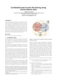
<strong>Speech</strong> (PoS) <strong>Tagging</strong>. <strong>Part</strong> <strong>of</strong> <strong>Speech</strong> tagging means tagging<br />
the words with their correct word classes.<br />
Figure 1. A tagged sentence.<br />
There are several ways <strong>of</strong> automatic tagging, which can be<br />
roughly divided in two main categories, rule based and<br />
stochastically based taggers. A rule based tagger tries to tag<br />
sentences according to handmade rules. Like after an article<br />
there will be a noun. This is just an example, <strong>of</strong> course this is<br />
not the complete rule, there can be adjectives between them.<br />
Building these rules requires much time and knowledge <strong>of</strong> the<br />
language. Stochastically based taggers do not use such rules;<br />
they compute the most likely tags for each word by learning<br />
lots <strong>of</strong> tagged sentences. These sentences, <strong>of</strong> course, must be<br />
tagged first, so lots <strong>of</strong> manpower is required. One example <strong>of</strong> a<br />
stochastically based tagger is a tagger based on hidden Markov<br />
models (HMM). It uses lots <strong>of</strong> data to compute and store lists <strong>of</strong><br />
Permission to make digital or hard copies <strong>of</strong> all or part <strong>of</strong> this work for<br />
personal or classroom use is granted without fee provided that copies<br />
are not made or distributed for pr<strong>of</strong>it or commercial advantage and that<br />
copies bear this notice and the full citation on the first page. To copy<br />
otherwise, or republish, to post on servers or to redistribute to lists,<br />
requires prior specific permission.<br />
4th Twente Student Conference on IT , Enschede 30 January, 2006<br />
Copyright 2006, University <strong>of</strong> Twente, Faculty <strong>of</strong> Electrical<br />
Engineering, Mathematics and Computer Science<br />
occurrences <strong>of</strong> words and combinations <strong>of</strong> tags. All these<br />
tagged sentences together are called the corpus. In this paper<br />
another stochastically based tagger is used, a tagger with a<br />
neural network.<br />
<strong>Neural</strong> networks were a big hype in the nineties. In many<br />
research areas neural networks were used. (Like character<br />
recognition, expert systems) In this period several studies for<br />
new ways <strong>of</strong> <strong>Part</strong> <strong>of</strong> <strong>Speech</strong> <strong>Tagging</strong> also used these neural<br />
networks. The last few years this interest diminished.<br />
For some specific areas (like jurisprudence) the existing taggers<br />
are not the best way. Building new taggers for these problems is<br />
expensive and needs a lot <strong>of</strong> manpower. But several documents<br />
[nak90, sch94] showed that only a small training corpus is<br />
enough for pretty good results. So reintroducing neural<br />
networks could perhaps save lots <strong>of</strong> money and manpower. This<br />
paper tries to answer the question if a tagger based on neural<br />
networks retrieve a high accuracy with small and large corpora<br />
build from the CGN corpus.<br />
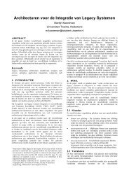
2. NEURAL NETWORKS<br />
A computer based neural network finds its origin in biology. It<br />
is a simple interpretation how biological neurons communicate<br />
with each other. Just like its biological counterparts, a computer<br />
neuron processes its input and passes its reaction onto another<br />
neuron. A biological neuron will fire if its inputs reach some<br />
threshold (bias) and will fire more when stimulated more. The<br />
computer neuron works almost the same, this is implemented<br />
with a so called bias neuron, describing the precise working is<br />
beyond the object <strong>of</strong> this paper, more information can be found<br />
at [nis03].<br />
W t -1 feat1<br />
W<br />
t -1<br />
feat2<br />
W<br />
t<br />
feat1<br />
W t feat2<br />
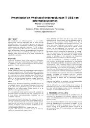
Input layer<br />
Hidden layer<br />
Output layer<br />
Figure 2. A neural network with one hidden layer<br />
Tag1<br />
Tag2<br />
The last ten years a couple <strong>of</strong> researchers studied the use <strong>of</strong><br />
neural networks for PoS (<strong>Part</strong> <strong>of</strong> <strong>Speech</strong>) taggers. Although<br />
they all differ quite a lot, one thing is always the same; they all<br />
use a feed forward network with back propagation. A feed<br />
forward network consists <strong>of</strong> a couple <strong>of</strong> input neurons, which<br />
pass their values onto a hidden layer, and every layer feeds its<br />
values into the next one, until it reaches the output layer. The
next equation shows the formulas. The input <strong>of</strong> n th neuron <strong>of</strong> the<br />
j th layer is the sum <strong>of</strong> the outputs <strong>of</strong> the layer before (layer j-1)<br />
times the weight between these neurons. Afterwards the<br />
standard sigmoid function is used to compute the output <strong>of</strong> this<br />
neuron. Neurons <strong>of</strong> the input layer do not use these formulas;<br />
their output is the input <strong>of</strong> the network.<br />
input<br />
j,<br />
n<br />
output<br />
= (<br />
output<br />
j,<br />
n<br />
i=<br />
# neuronsLayer<br />
1<br />
=<br />
1+<br />
e<br />
−input<br />
j−1<br />
j , n<br />
j−1,<br />
i<br />
* weight<br />
j,<br />
n,<br />
i<br />
Equation 1. Computation <strong>of</strong> the output <strong>of</strong> a neuron<br />
In the output layer every neuron fires between 0 and 1, because<br />
<strong>of</strong> this output function. The neuron with the highest output<br />
value will be the winner and its number represents the number<br />
<strong>of</strong> the tag. When the training <strong>of</strong> the network starts all the<br />
weights in the network get a random value, so the outcome will<br />
probably not match with the desired output. During the training<br />
<strong>of</strong> the network, the network computes the output (Feed<br />
forward). Then, with the desired output, adjusting the weights<br />
backwards, starting with the weights on the output layer<br />
finishing with the weights between the input layer and the first<br />
hidden layer (back propagation). The network will learn how to<br />
react properly on input by training all the data several times in a<br />
row. The power <strong>of</strong> neural networks is the fact that slightly<br />
different input will result in the same output, samples almost the<br />
same. [her91]<br />
2.1 Layers <strong>of</strong> the Network<br />
Some <strong>of</strong> the studies done by others differ in the use <strong>of</strong> hidden<br />
layers. One <strong>of</strong> the earliest studies [nak90] contained networks<br />
with two hidden layers. This made the networks quite complex.<br />
Later studies by Schmidt [sch94] and Marques [mar01] proved<br />
that such complex networks do not pay <strong>of</strong>f. Marques compared<br />
a network without a hidden layer (only an input and output<br />
layer) to a network with a hidden layer and concluded that the<br />
first one was easier to train and reached a higher accuracy.<br />
2.2 Input Features<br />
The main difficulty with a neural network is the question what<br />
to use as input. Boggess [bog92] tried several features, like<br />
mapping the last letters <strong>of</strong> the words on the input neurons, and<br />
another method by representing all the words with a number<br />
and feeding this binary to the input neurons. All methods<br />
seemed useless. The recognition was bad and results differed<br />
greatly between the test runs. Boggess concluded his approach<br />
was not the right one. The only workable way found is feeding<br />
the network with a number <strong>of</strong> tags. This is done by a sliding<br />
window; this means the network can compute one tag at a time,<br />
for every word in the sentence the network will be fed with zero<br />
or more tags back, the current word and zero or more words<br />
ahead. Figure 2 shows a network with two tags and a sliding<br />
window <strong>of</strong> 2. The current word t and the previous word t-1 are<br />
fed, so the next step will be to fed word t+1 as current word and<br />
word t as previous word. This is a very small network, with a<br />
sliding window <strong>of</strong> size six tags and over 70 different tags, the<br />
input layer will contain over 400 neurons. Both Schmidt and<br />
Marques uses a lexicon with relative frequencies <strong>of</strong> the tags per<br />
word stored. These relative frequencies are fed to the input<br />
neurons. Feeding the network three words requires three times<br />
the number <strong>of</strong> tags from the tagset input neurons. All the<br />
approaches differ in the size <strong>of</strong> the sliding window, Marques<br />
uses a window <strong>of</strong> three words and Schmidt a window <strong>of</strong> six<br />
)<br />
words. Some [nak90] use their results found for word n as input<br />
for word n+1. So instead <strong>of</strong> the relative frequencies <strong>of</strong> the tags<br />
<strong>of</strong> the words before, the network gets the computed values <strong>of</strong><br />
the tags before. This is more difficult to train, but can improve<br />
the recognition. Knowledge <strong>of</strong> the previous tags improves the<br />
recognition <strong>of</strong> the tags <strong>of</strong> the next words.<br />
2.3 Output <strong>of</strong> the network<br />
Because every network processes one word at a time the output<br />
is also one tag at a time. This can be done in two ways. One<br />
method is to give every output neuron its own tag, so there are<br />
as many output neurons as there are tags in the tagset [sch94].<br />
The output neuron with the highest output value indicates the<br />
most likely tag. Another way is to number the tags and let the<br />
output neurons hold the binary representation <strong>of</strong> this number<br />
[bog92]. The second one saves a lot <strong>of</strong> output neurons, for<br />
example 89 tags can be numbered with 7 bits, giving 7 output<br />
neurons, all representing one bit when giving an output above<br />
some threshold. But there are some major disadvantages in<br />
this coding. With the first method there is always a neuron<br />
firing the most. The network will choose between two likely<br />
candidates. With the second one a small error may result in a<br />
totally different tag when one neuron is just a bit above<br />
threshold. It could very well give some kind <strong>of</strong> logical AND <strong>of</strong><br />
the most likely tags, giving a totally different tag number. This<br />
makes it much more difficult to train.<br />
2.4 Final Remarks on <strong>Neural</strong> <strong>Networks</strong><br />
The term learning rate occurs in the field <strong>of</strong> neural networks as<br />
well in the field <strong>of</strong> <strong>Part</strong> <strong>of</strong> <strong>Speech</strong> tagging. In the field <strong>of</strong> neural<br />
networks this means how much the weights <strong>of</strong> the network can<br />
change in one training step. A large learning rate results in a<br />
quick learning, but will not result in an overall best network (a<br />
local optimum). A small learning rate takes longer to train, but<br />
will end more easily in a stable, good network. Therefore a<br />
normal learning rate is used to make the network more stable.<br />
In PoS tagging the learning rate is the relation between the size<br />
<strong>of</strong> the corpus and the accuracy the tagger achieves. The learning<br />
rate shows how much the accuracy increases when the amount<br />
<strong>of</strong> training data grows. Another issue is over-learning. A neural<br />
network is powerful because it is able to compute answers to<br />
unseen samples. If a sample is more or less the same as another<br />
sample it will react the same. So the network will produce good<br />
results on slightly different input. But if the network is too large<br />
(to many hidden layers, to many neurons in the hidden layer), it<br />
will learn the samples instead <strong>of</strong> the bigger picture. A final<br />
remark must be made about the computation time. The larger<br />
the net, the more weights it contains, the longer it will take to<br />
compute an answer. Fortunately the computers today are<br />
powerful enough to process lots <strong>of</strong> data. Some years ago the<br />
computing speed would make it impossible to train as many<br />
nets as it would today. [sch94] claims he needs one day <strong>of</strong><br />
computation power on a sparc10 for the training <strong>of</strong> a 2 million<br />
words corpus. But today, with a relatively slow computer<br />
(Athlon 2500+) one is able to test 1 million words with a large<br />
network in less than 2 minutes.<br />
3. RESEARCH QUESTIONS<br />
Considering the problems mentioned in the introduction the<br />
main question will be:<br />
Will the promising results for other languages (good tagging<br />
with small corpora) also hold for <strong>spoken</strong> <strong>Dutch</strong> <strong>Part</strong> <strong>of</strong> <strong>Speech</strong><br />
tagging <strong>using</strong> the CGN corpus
3.1 Derived Research Questions<br />
The main question can not be answered without a few other<br />
questions.<br />
• Structure. Are the structures <strong>of</strong> the neural networks found<br />
in the literature [nak90, sch94] efficient for <strong>spoken</strong> <strong>Dutch</strong><br />
texts<br />
• Input features. What are the best features for input<br />
neurons What size <strong>of</strong> the sliding window gives the best<br />
result<br />
• Accuracy. How does a neural network approach perform<br />
compared to other Taggers In particular how does<br />
perform compared to a HMM tagger and a Support Vector<br />
Machine tagger [lui05]<br />
• Learning rate. Many reports, like the report <strong>of</strong> Marques<br />
[mar01], claim that neural network have a very good<br />
learning rate, will these results hold for the CGN corpus<br />
4. LEXICON AND CORPUS<br />
Like all stochastic taggers, a neural network needs a lexicon<br />
with per word a list <strong>of</strong> possible tags with their relative<br />
frequencies. There are two ways to build this lexicon:<br />
• Make the lexicon as large as possible; use external<br />
lexicons with relative word frequencies, use all the tagged<br />
texts available. This should make the best list <strong>of</strong><br />
occurrences <strong>of</strong> words.<br />
• Use only the words and tags from the training corpus, this<br />
gives a less complete lexicon. But results give a better<br />
view <strong>of</strong> the performance <strong>of</strong> the tagger, instead <strong>of</strong> the<br />
quality <strong>of</strong> the lexicon [mar01].<br />
Marques [mar01] shows that the first one gives the best results<br />
with very small subsets (with only 10.000 words the results are<br />
almost at a maximum). This is obvious <strong>of</strong> course, the second<br />
one did not see that many words, its lexicon will not have a well<br />
built list with relative frequencies.<br />
4.1 The Corpus Gesproken Nederlands<br />
The CGN (Corpus Gesproken Nederlands) corpus is a large<br />
corpus, based on <strong>spoken</strong> <strong>Dutch</strong>. [cgn04] The whole corpus is<br />
around 9.000.000 words, divided in 15 different sections.<br />
Mentioned in the table 1.<br />
The choice <strong>of</strong> <strong>using</strong> the CGN got some implications.<br />
• The CGN corpus is built out <strong>of</strong> normal <strong>spoken</strong> sentences,<br />
so not every sentence in the corpus will be correct <strong>Dutch</strong>,<br />
making tagging a bit harder.<br />
• The CGN corpus is filled with <strong>Dutch</strong> <strong>spoken</strong> by people<br />
from the Netherlands and Belgium. There are some<br />
differences between those two dialects. Like sometimes the<br />
words are put in a different order, for example in the<br />
Netherlands people say: “vast en zeker” And in Belgium<br />
people use it the other way around: “zeker en vast”. (It<br />
means “for sure”). One third <strong>of</strong> the corpus is Flemish, the<br />
rest <strong>Dutch</strong> <strong>spoken</strong> by people from the Netherlands. No<br />
tests are done with the different dialects.<br />
This data is distributed over eleven files, putting the first line in<br />
file one the second in file two and so on. This makes the data<br />
equally spread over the eleven files. All testing is done on file<br />
one, called set0. Because <strong>of</strong> the large size <strong>of</strong> the corpus (all files<br />
contains over 100.000 sentences) most <strong>of</strong> the experiments are<br />
done with just one or two <strong>of</strong> the files for training. This will be<br />
mentioned for each test.<br />
Data<br />
Table 1. Overview <strong>of</strong> the corpus<br />
Size<br />
(in words)<br />
A Face to face conversations 2626172<br />
B Interviews with teacher <strong>Dutch</strong> 565433<br />
C Phone dialogue (recorded at platform) 1208633<br />
D Phone dialogue (recorded with mini disc) 853371<br />
E Business conversations 136461<br />
F<br />
Interview & discussions record from<br />
radio<br />
790269<br />
G Political debates, discussions & meetings 360328<br />
H Lectures 405409<br />
I Sport comments 208399<br />
J Discussion on current events 186072<br />
K News 368153<br />
L Comments on radio & TV 145553<br />
M Masses, ceremonies 18075<br />
N Lectures, discourses 140901<br />
O Texts, read aloud 903043<br />
4.2 The Tagset<br />
The CGN corpus is tagged with a large tagset [Eyn04] <strong>of</strong> 316<br />
tags. This tagset can easily be simplified to a smaller tagset.<br />
This simplification is done by grouping <strong>of</strong> tags. There are three<br />
main tagsets:<br />
• The large tagset. This is a really large tagset, compared to<br />
the Brown tagset (87) and the Penn Treebank tagset (48).<br />
Because <strong>of</strong> its size many tags are rarely used. Although the<br />
CGN corpus is a large corpus, some tags occur only once,<br />
making the training and recognizing <strong>of</strong> these tags very<br />
difficult.<br />
• The medium tagset. This reduced set <strong>of</strong> 72 tags is derived<br />
from the larger set <strong>of</strong> 316 tags by grouping tags that look<br />
alike. The reduced set <strong>of</strong> 72 tags makes, for example, no<br />
difference between the seven articles described in the<br />
original set. But does not group all the verbs to one tag, it<br />
still uses, for example, the difference between normal<br />
verbs and auxiliary verbs.<br />
• The small tagset. With this tagset the number <strong>of</strong> tags is<br />
reduced even further, leaving one with only the twelve<br />
main tags, like verb, noun.<br />
At the start <strong>of</strong> this project the first intention was to use a tagset<br />
with twelve tags, but after a few tests this tagset seemed to be<br />
too small. The base tagger (simply returning the most used tag)<br />
produced a result <strong>of</strong> over 95%. This leaves no room for<br />
improvement. Using the 72 tags sized tagset the base tagger<br />
recognized around 91%. This leaves enough errors to make a<br />
better tagger. This larger tagset splits the main categories in<br />
more precise tags. For example it splits the tag VG<br />
(conjunction) in subordinating conjunction and coordinating<br />
conjunction. More about the CGN-tagset can be found in<br />
[Eyn04].
Even in this 72 tagset there are quite a number <strong>of</strong> tags hardly<br />
used. VNW10, N8, VNW18, VNW4, WW5, VNW9, ADJ8<br />
occur less than 100 times and half the tagset occurs less than<br />
10.000 times. With over a 10,000,000 words, their occurrences<br />
are very rare. In total these 36 tags are 1.2% <strong>of</strong> the whole<br />
corpus.<br />
Table 2. The different tags <strong>of</strong> the 72 tagset<br />
Tag numbers <strong>Part</strong> <strong>of</strong> <strong>Speech</strong> tag Tags in CGN corpus<br />
1…8 Noun N1, N2… N8<br />
9…21 Verb WW1, WW2… WW13<br />
22 Article LID<br />
23…49 Pronoun VNW1…VNW27<br />
50, 51 Conjunction VG1, VG2<br />
52 Adverb BW<br />
53 Interjections TSW<br />
54...65 Adjective ADJ1…ADJ12<br />
66…68 Preposition VZ1,VZ2,VZ3<br />
69,70 Numeral TW1, TW2<br />
71 Punctuation LET<br />
72 Special SPEC<br />
Table 3 shows the most occurring tags. Together these 12 tags<br />
occupy over 70% <strong>of</strong> the whole corpus. Notice that 3% <strong>of</strong> the<br />
corpus is tagged with SPEC, meaning 3% <strong>of</strong> the words in the<br />
corpus are special cases. This tag is used for unfinished words,<br />
noises like coughing and words from foreign languages. Most<br />
<strong>of</strong> these cases occur because the CGN corpus is built out <strong>of</strong><br />
<strong>spoken</strong> <strong>Dutch</strong> sentences.<br />
Table 3. Overview <strong>of</strong> the most frequently used tags<br />
Number Tag % number tag %<br />
71 LET 11,2 22 LID 5,3<br />
52 BW 10,4 23 VNW1 4,9<br />
53 TSW 7,8 50 VG1 4,0<br />
1 N1 7,4 62 ADJ9 3,4<br />
9 WW1 6,7 72 SPEC 3,0<br />
66 VZ1 6,7 12 WW4 2,6<br />
5. EXPERIMENT SETUP<br />
Reading about neural networks, the target looks very easy, but<br />
contains a lot <strong>of</strong> choices. In this section all the different choices<br />
are presented.<br />
5.1 The Trained networks<br />
The questions mentioned in the section 3 require lots <strong>of</strong><br />
different tests. This section shows these different kinds <strong>of</strong> tests,<br />
split in a few categories:<br />
• Testing the window size. It is important to know what the<br />
influence is <strong>of</strong> increasing the window size. A window size<br />
<strong>of</strong> one is the normal base tagger. Knowing more words<br />
before and after the current word will improve the<br />
accuracy, but to what extent.<br />
• Testing the influence <strong>of</strong> a hidden layer. When adding a<br />
hidden layer the network will be able to see more complex<br />
relations. Marques [Mar01] concluded that adding a hidden<br />
layer did not improve the recognition. A few networks will<br />
be tested to verify his findings.<br />
• Testing different kinds <strong>of</strong> input. As mentioned in section<br />
2.2, neural networks work the best when it is fed with tags.<br />
But which tags gives the best performance When the<br />
tagger uses a window size <strong>of</strong> two words back, two words<br />
ahead and it is tagging the third word should it use the<br />
relative frequencies <strong>of</strong> the tags found in the lexicon or<br />
should it use the computed tags And when <strong>using</strong> the<br />
second method will it make more errors After all, if it<br />
makes a mistake with the first word, it will use a wrong tag<br />
to predict the next. A few tests are done to determine if<br />
there is a best way.<br />
• Testing the learning rate. One <strong>of</strong> the main questions is:<br />
Will a neural network perform well with a small corpus<br />
To test this, different kinds <strong>of</strong> networks with different<br />
sized corpora are used.<br />
• How to handle unknown words. Unknown words are a<br />
problem for all existing taggers, some tests must determine<br />
how to handle unknown words.<br />
• Building the best network. Of course one always wants to<br />
find the best network possible. During these tests all the<br />
results <strong>of</strong> the other test are used to construct the network<br />
with the highest accuracy possible.<br />
Because <strong>of</strong> the many parameters not every networks possible<br />
with the questions above can be built. The five tests above<br />
contain to many parameters to build all the combinations<br />
possible.<br />
5.2 Comparing the Results with Other<br />
Taggers<br />
Before any conclusions about the performance can be made,<br />
there must be some comparison with other taggers. During these<br />
tests two other taggers are used as reference. The first one is the<br />
base tagger; it stores all the words with their tags <strong>of</strong> the training<br />
corpus. Afterwards all the words <strong>of</strong> the test corpus are tagged<br />
with the highest frequency <strong>of</strong> a tag for that word. (Example: the<br />
<strong>Dutch</strong> word “een” can be an article or a numeral (meaning the<br />
word one), in most <strong>of</strong> the cases it is an article (meaning the<br />
word a), so tag it with article). The second tagger is a HMM<br />
(Hidden Markov Model) tagger with bigrams. It stores tuples <strong>of</strong><br />
tags and their frequencies and tries to match this with the test<br />
set. Only the bi-grams are used, the complexity (memory use,<br />
computation time) <strong>of</strong> larger n-grams grows rapidly, which<br />
makes it a research area on its own.<br />
6. RESULTS<br />
According to the literature the best performance was obtained<br />
with a network with a window size <strong>of</strong> six, three words back, the<br />
word itself and two words ahead. [sch94]. This will be the base<br />
<strong>of</strong> many <strong>of</strong> the tests.<br />
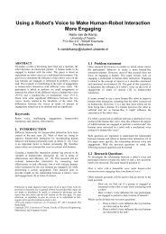
6.1 Test 1: The Window Size<br />
The first target is to verify the results found by [mar01] and<br />
[sch94], they claimed that a neural network with a window size<br />
<strong>of</strong> six, three tags back, the relative frequencies <strong>of</strong> the tags <strong>of</strong> the<br />
word, and two tags ahead. In the next tests the next notation is<br />
used: bxa, where b is the number <strong>of</strong> tags back and a the number<br />
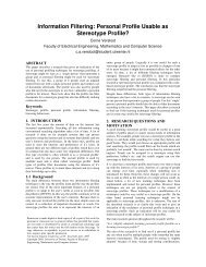
<strong>of</strong> tags ahead. So this network will be called 3x2. The figure<br />
below shows 7 different networks. These networks are trained<br />
with 1 file from the trainings set and tested with the test file,<br />
set0. The X-axis shows the number <strong>of</strong> times all the samples are<br />
trained.
96,3<br />
96,2<br />
96,1<br />
96<br />
95,9<br />
base<br />
1x4<br />
3x2<br />
4x1<br />
1x1<br />
2x2<br />
3x3<br />
4x4<br />
95,8<br />
1 3 5 7 9 11<br />
Figure 3. Influence <strong>of</strong> the Window Size<br />
The difference between the nets seems pretty obvious, but<br />
notice there is only an area <strong>of</strong> .4% in which all the nets perform.<br />
The base tagger results in an accuracy <strong>of</strong> 91.8%, so all the<br />
neural networks perform much better. (The results <strong>of</strong> the base<br />
tagger can not be seen in the figure) Because <strong>of</strong> the small<br />
differences between all the nets the next tests use the network<br />
preferred by the literature. [sch94]<br />
96,6<br />
96,58<br />
96,56<br />
96,54<br />
96,52<br />
96,5<br />
96,48<br />
96,46<br />
3x2<br />
1mil 2mil 3mil 4mil<br />
Figure 4. A long run with a 3x2 network<br />
Figure 4 shows the influence <strong>of</strong> a longer run. This time all the<br />
data is used, and this is fed one, two, three and four times to<br />
network. Feeding the network multiple times with the data does<br />
improve its recognition, but the graph flattens within three to<br />
four cycles.<br />
6.2 Test 2: Hidden Layers<br />
To test the influence <strong>of</strong> a hidden layer a bit more data is used,<br />
because the networks are more complex. This time 2 files <strong>of</strong> the<br />
training data are used. Each network is fed with 400000 lines<br />
from this data.<br />
Shape<br />
Table 4. The influence <strong>of</strong> a hidden layer<br />
Result<br />
3x2 hidden layer 30 95,69<br />
3x2 hidden layer 40 95,91<br />
3x2 hidden layer 60 96,17<br />
3x2 hidden layer 73 96,10<br />
3x2 hidden layer 100 95,98<br />
Because the complexity <strong>of</strong> the net, which may result in<br />
suboptimal networks, this test is done twice. After these tests<br />
the results did not differ that much. (Less than 0.2%). The<br />
average results are presented in Table 4. These results show that<br />
a small hidden layer has a negative effect on the results. The<br />
best network seems to be the network with 60 neurons. Nets<br />
with larger hidden layers possibly suffer from over-learning.<br />
6.3 Test 3: What Input To Use<br />
While trying to build the best network possible (see section<br />
6.7), one question was what input data to use. The data can be<br />
trained in different ways:<br />
• Method 1. Always feed the relative frequencies <strong>of</strong> the tags<br />
possible for each word. Using a 3x2 network would be fed<br />
with the relative frequencies <strong>of</strong> the tags three words back,<br />
the relative frequencies <strong>of</strong> tags <strong>of</strong> the word itself and those<br />
<strong>of</strong> the two words ahead.<br />
A positive effect is that the wrong recognition <strong>of</strong> a word<br />
would not affect the next.<br />
A negative effect is that the results <strong>of</strong> the tags already<br />
found are not used. If the tagger is correct <strong>using</strong> its answer<br />
will be better than the relative frequencies <strong>of</strong> tags <strong>of</strong> this<br />
word.<br />
• Method 2. Feeding the network with relative frequencies<br />
<strong>of</strong> the tags <strong>of</strong> the current words and the two words ahead,<br />
but use the found tags <strong>of</strong> the words back. In this case<br />
during the training the desired tags <strong>of</strong> the words back can<br />
be fed.<br />
This method has exactly the opposite effects, a wrong<br />
recognition affects the next word and a good prediction<br />
strengthens the next prediction.<br />
Another positive effect is that a neural network never<br />
really fires at one neuron alone. There is always a second<br />
best. Using all the output <strong>of</strong> the last word gives the<br />
network a change to benefit <strong>of</strong> it. But here is another<br />
problem, during training only the desired tag is fed. (Can<br />
one think <strong>of</strong> a second best, when one knows the correct<br />
answer) During testing it will see data it has never seen<br />
before. But giving only the most firing tag will increase the<br />
power <strong>of</strong> an error onto the next tag.<br />
• Method 3. A mixture <strong>of</strong> both. Feeding the network with the<br />
relative frequencies and the outcome <strong>of</strong> the last recognition<br />
is also an option. During training it will see the influence<br />
<strong>of</strong> the correct tag <strong>of</strong> the last word, but also the existence <strong>of</strong><br />
a second best (the other tags possible) and will learn this<br />
extra information.<br />
Table 5 shows the results <strong>of</strong> the 3 described ways.<br />
Table 5. Testing different kinds <strong>of</strong> input<br />
Input used After 1 run After 2 runs<br />
Tags only 96,27 96,55<br />
Computed results only 96,37 96,50<br />
Tags and computed results 96,40 96,55<br />
These results may seem a bit difficult to explain. First <strong>of</strong> all<br />
notice that the differences are not that large. After the first run<br />
the network is clearly not finished learning, and it shows that<br />
the network finds it a bit more difficult to figure out which tag<br />
to use, so tags only produces a slightly worse output. Using the<br />
output only lets the network produce results more easily, after<br />
one run it works better than the first. After the second run the<br />
chances have changed. The network knows better how to
handle more tags on the input. And the good results <strong>of</strong> only<br />
<strong>using</strong> the computed results are punished with more errors after<br />
two runs. The mixture shows the best <strong>of</strong> both worlds. And<br />
although the differences are small, from this point on the<br />
mixture input is used. It is merely done because it seems to get<br />
better results with less data.<br />
6.4 Test 4: Different Size <strong>of</strong> Corpora<br />
In the literature all papers mention the good learning rate <strong>of</strong><br />
<strong>Part</strong> <strong>of</strong> <strong>Speech</strong> taggers based on neural networks [mar01].<br />
Because the CGN-corpus is rather large, this has to be split in a<br />
few subparts to test the learning rate. The tests are done with<br />
three small parts from one training file, a part containing the<br />
first 100 lines, one with 1000 lines and a third with 10000 lines.<br />
The training data all come from the face to face conversation,<br />
so it is tested with the face to face conversation part <strong>of</strong> the test<br />
files. Below are the results <strong>of</strong> the 100 line corpus.<br />
75<br />
74<br />
73<br />
72<br />
71<br />
70<br />
69<br />
68<br />
67<br />
Base<br />
1x1<br />
2x2<br />
3x2<br />
66<br />
3x3<br />
4x4<br />
65<br />
3x3x60<br />
3x3x100<br />
0 5 10 15 20 25 30<br />
Figure 5. Learning a 100 lines corpus<br />
It is clear that this training set is too small, the training data had<br />
to be fed 20 times (makes 2000 lines) to get near the base<br />
tagger. After 20 times only 100 lines (whole trainings corpus)<br />
the tests are stopped. At this point the program produced output<br />
every 2000 lines, to get the best tagger possible. After around<br />
20000 times one <strong>of</strong> the 100 lines trained the network stopped<br />
learning (it flattens). The figure shows clearly that adding a<br />
hidden layer results in a lower performance.<br />
85<br />
84<br />
83<br />
82<br />
Base<br />
1x1<br />
2x2<br />
3x2<br />
3x3<br />
4x4<br />
81<br />
3x3x60<br />
3x3x100<br />
2 7 12 17 22 27<br />
Figure 6. Learning a 1000 lines corpus<br />
Next the 1000 line corpus is trained. Every 1000 lines the<br />
program produces output, and after around 20000 times a line<br />
from the corpus the output flattens, showing the network<br />
reaches its maximum. This figure shows clearly that all the<br />
networks perform better than the base tagger. It also shows that<br />
with such a small corpus the choice <strong>of</strong> which network is<br />
irrelevant. Only the ones with hidden layers don not perform<br />
well. They keep bouncing around.<br />
92,4<br />
92,2<br />
92<br />
91,8<br />
91,6<br />
91,4<br />
91,2<br />
91<br />
Base<br />
2x2<br />
3x3<br />
3x3x60<br />
1x1<br />
3x2<br />
4x4<br />
3x3x100<br />
1 6 11 16 21<br />
Figure 7. Learning a 10000 lines corpus<br />
The next test used a 10000 lines corpus. And again the program<br />
produces output when the whole corpus is trained once, so after<br />
10000 lines. After 200.000 times training a line (20 times this<br />
corpus) the output flattens, showing that the best network<br />
results in recognition <strong>of</strong> around 92.2% for a 3x2 network. The<br />
base tagger performs only 88.4% and can not be seen in the<br />
figure.<br />
These three tests make clear that a corpus can be too small for a<br />
good tagger. A training set <strong>of</strong> 100 lines is way too small to get a<br />
good tagger. Above 1000 lines the networks performs<br />
significant better than a base tagger. With small corpora the use<br />
<strong>of</strong> a hidden layer is a very wrong choice. The results do not<br />
stabilize quickly and when stabilized are significant below the<br />
results <strong>of</strong> the networks without hidden layer. This may be a<br />
result <strong>of</strong> over-learning; it is learning the specific sentences,<br />
instead <strong>of</strong> the big picture.<br />
To complete the tests <strong>of</strong> the influence <strong>of</strong> larger corpora another<br />
test is done. While searching for the best network (section 6.7),<br />
it showed that a hidden layer can improve the recognition. The<br />
next test is done with a 3x2 network with a hidden layer <strong>of</strong> 60<br />
neurons because <strong>of</strong> the good results (see section 6.2). To<br />
remove the effect <strong>of</strong> a better lexicon, the following tests are<br />
done with a lexicon built <strong>of</strong> all the trainings data. First a<br />
network is trained <strong>using</strong> two files (a 200000 lines corpus). This<br />
network is fed 800000 times with one line. This resulted in a<br />
recognition <strong>of</strong> 96,9% Afterwards the network is copied, making<br />
two identical Nets. Network1 is fed with the same corpus<br />
400000 times. Network2 gets a new corpus with the next two<br />
files (again a 200000 lines corpus) and is fed with 400000 times<br />
one line. Again Network2 is copied, making two identical Nets,<br />
Network2a and Network2b. Network1 is fed again with 400000<br />
lines from the first corpus, Network2a again with the second<br />
corpus. Network2b is fed with a third corpus, again another two<br />
files (again 200000 lines). So every network is trained with<br />
exactly the same number <strong>of</strong> lines. Table 6 shows the results.<br />
These results show clearly that increasing the corpus does not<br />
improve the recognition much. Using a 3 times larger corpus
improves the recognition by 0.03%. Of course this small<br />
improvement is used in section 6.7 to try to build the best<br />
network.<br />
Table 6. Influence <strong>of</strong> a larger corpus<br />
Network Trainings set Recognition<br />
Network1 1,6 million lines from a 200000<br />
line corpus<br />
Network2a 1,6 million lines from a 400000<br />
line corpus<br />
Network2b 1,6 million lines from a 600000<br />
line corpus<br />
96,97%<br />
96,99%<br />
97,00%<br />
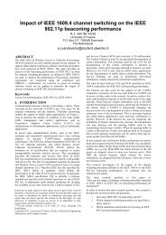
6.5 Unknown Words<br />
Giving unknown words the correct tags is a study on its own.<br />
And this is not the objective <strong>of</strong> this paper. To get some idea <strong>of</strong><br />
the kinds <strong>of</strong> unknown words the trainings corpus is split into ten<br />
parts. Every time a lexicon <strong>of</strong> nine parts was build and the tenth<br />
part was used to count the occurrence <strong>of</strong> the tags <strong>of</strong> the<br />
unknown words. This test was done ten times every time <strong>using</strong><br />
another subset to count the unknown word tags. Of course the<br />
test set is not used at all, this remains the testing candidate. It<br />
should not be used to optimize the results.<br />
opposite is true for N3 and N5, they do not occur very <strong>of</strong>ten in<br />
the whole corpus (less than 2%) but they are important tags for<br />
the unknown words.<br />
Now the network can be fed with these relative frequencies<br />
instead <strong>of</strong> an equal weight <strong>of</strong> 1/72 for every input neuron. This<br />
should help the network with the recognition <strong>of</strong> these unknown<br />
words. A small test showed that this way <strong>of</strong> handling unknown<br />
words is better than a 1/72 weight to all the inputs. With the use<br />
<strong>of</strong> a 3x2 network 10.000 trainings sentences the results were<br />
92.4% for a weighted distribution and 91.7% with an equal<br />
spread. The next tests all will be done with these relative<br />
frequencies in stead <strong>of</strong> an equal weight for every input neuron.<br />
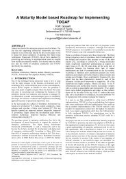
6.6 Comparing <strong>Neural</strong> <strong>Networks</strong> with the<br />
base tagger and the HMM tagger<br />
According to the results in the previous sections a tagger can be<br />
built with the use <strong>of</strong> a neural network, but how well does it<br />
perform compared to other taggers During this test the results<br />
<strong>of</strong> the neural network trained in preceding tests are plotted<br />
against the results <strong>of</strong> a base tagger and the HMM tagger. The<br />
HMM tagger is trained with Simple Good-Turing context<br />
smoothing and Witten-Bell lexical smoothing. The neural<br />
network used is a 3x2 network.<br />
Occurence (%)<br />
40<br />
35<br />
30<br />
25<br />
20<br />
15<br />
10<br />
5<br />
10 9 8 7<br />
6 5 4 3<br />
2 1 GEM<br />
0<br />
0 20 40 60<br />
Tag number<br />
Figure 8. Spreading <strong>of</strong> the unknown tags<br />
Every part added roughly around 8900 new unknown words.<br />
The frequencies <strong>of</strong> the tags over these sets also did not differ a<br />
lot. (Notice that in the next figure the ten dots are so close, they<br />
look like a single dot) All the tags are numbered with the<br />
numbers mentioned in section 4.2. Only the tags with an<br />
occurrence <strong>of</strong> at least 2% are used to predict unknown words.<br />
These nine tags cover over 90% <strong>of</strong> the words.<br />
Table 7. The largest frequencies <strong>of</strong> the tags <strong>of</strong> unknown<br />
words<br />
Tag<br />
Nr<br />
Tag Freq Tag<br />
Nr<br />
Tag<br />
Freq<br />
1 N1 33% 15 WW7 2,5%<br />
3 N3 14% 54 ADJ1 4,0%<br />
5 N5 10% 62 ADJ9 2,4%<br />
9 WW1 2,2% 72 SPEC 19%<br />
12 WW4 2,3%<br />
Notice the differences between this table and table 3. Although<br />
TSW and BW occur quite a lot (see table 3) and they are both<br />
open word classes, they do not occur in the table above. The<br />
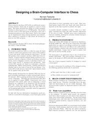
performance<br />
100<br />
95<br />
90<br />
85<br />
80<br />
75<br />
70<br />
65<br />
Base<br />
HMM<br />
60<br />
100 1000 10000 100000 1000000<br />
corpus size<br />
Figure 9. Results <strong>of</strong> a neural network, a base and a HMM<br />
tagger<br />
One can clearly see that neural network gives much better<br />
results. Especially with small corpora, the differences are over<br />
five percent. So the findings <strong>of</strong> Marques [mar01] and others are<br />
also true for the CGN corpus.<br />
6.7 Building the best network<br />
After all these tests, all the information is used to build the best<br />
neural network possible, once more five <strong>of</strong> the most promising<br />
networks are trained. The results <strong>of</strong> the other tests are used to<br />
improve the best network found so far. Surprisingly the best<br />
net, found after many tests, was a network with a hidden layer.<br />
With use <strong>of</strong> all the improvements <strong>of</strong> the previous sections and<br />
the whole corpus the following results were achieved.<br />
With all the data available, a larger network seems to perform<br />
slightly better, like mentioned in [sch94]. But the results seem<br />
to differ more than one would expect according to the report <strong>of</strong><br />
Schmidt [sch94]. The results after adding a hidden layer are<br />
around 0.4% better, this is a rather large gain.<br />
NN
97,4<br />
97,3<br />
97,2<br />
97,1<br />
97<br />
96,9<br />
96,8<br />
3x3<br />
4x4<br />
3x3x60<br />
4x4x60<br />
3x3x100<br />
96,7<br />
0 2 4 6 8<br />
Figure 10. Search for the best network<br />
Figure 10 shows a 3x3 neural network with a hidden layer <strong>of</strong><br />
100 neurons got the best recognition. This network is used to<br />
compare the results <strong>of</strong> a neural network with a Support Vector<br />
Machine based tagger.<br />
Table 8 shows the results <strong>of</strong> the different parts <strong>of</strong> the corpus.<br />
All the test corpora are parts <strong>of</strong> set0, the test file. Every test is<br />
done with the first 10.000 lines <strong>of</strong> each part. (If possible, the<br />
corpus contains for example a part with Masses, ceremonies,<br />
but there are only 18075 lines in the total corpus. These lines<br />
are distributed over the 11 files. Meaning there are only around<br />
1500 lines <strong>of</strong> this part in set0.)<br />
Data<br />
Table 8. Results <strong>of</strong> the best network trained<br />
Results<br />
NN<br />
Results<br />
SVM<br />
Face to face conversations 97.3% 97.4%<br />
Interviews with teacher <strong>Dutch</strong> 97.1% 97.1%<br />
Phone dialogue (recorded at platform) 98,0% 98.0%<br />
Phone dialogue (recorded with mini<br />
disc)<br />
98.0% 98,0%<br />
Business conversations 97.8% 97,6%<br />
Interview & discussions record from<br />
radio<br />
96.9% 96,7%<br />
Political debates & discussions 96.5% 96,2%<br />
Lectures 97.3 % 97,2%<br />
Sport comments 97.3% 97,3%<br />
Discussions on current events 97,2% 97,2%<br />
News 96.7% 96,7<br />
Comments (radio, TV) 96.3% 95,7%<br />
Masses, ceremonies 95.5% 95,6%<br />
Lectures, discourses 96.3% 96,0%<br />
Texts, read aloud 96.2% 96,4%<br />
Total result <strong>of</strong> set0 97.3% 97,3%<br />
Table 8 not only the results <strong>of</strong> a tagger <strong>using</strong> neural networks<br />
are presented, but also the results <strong>of</strong> Luite Stegeman are shown.<br />
He built a tagger <strong>using</strong> Support Vector Machines [ste05]. His<br />
results are almost identical to the results <strong>of</strong> this paper. At some<br />
points this program gets better results, other parts are slightly<br />
better done with a neural network. The table shows that parts <strong>of</strong><br />
the CGN corpus with not that many lines (see Table 1 for the<br />
size <strong>of</strong> each part) do not perform very well. The neural network<br />
and the SVM tagger both tend to recognize the larger parts<br />
much better.<br />
Table 9. Overall performances <strong>of</strong> different taggers<br />
Tagger Results <strong>Tagging</strong> speed<br />
Support Vector Machines 97,3 1000<br />
Genetic Tagger 90,0 3000<br />
neural networks 97,3 7500<br />
The results <strong>of</strong> the two stochastical taggers are better than the<br />
Genetic tagger, built by Wouter Joosse. But the research done<br />
by Wouter Joosse [joo05] had a slightly different objective; he<br />
wanted to test if a Brill tagger can be simplified by <strong>using</strong><br />
Genetic algorithms.<br />
6.8 Error Analysis<br />
In this section the errors made by the tagger in section 6.7 are<br />
briefly mentioned. The next table shows the largest errors the<br />
network made. The network in section 6.7 reaches a recognition<br />
<strong>of</strong> 97,3%, so the error rate is 2,7%.<br />
Table 10. The largest errors<br />
Tag Occur Errors Recall Precision F 1<br />
WW2 17247 2018 0.88 0.92 0.90<br />
N3 19662 1615 0.92 0.98 0.95<br />
SPEC 27295 1582 0.94 0.93 0.93<br />
WW4 24005 1529 0.94 0.90 0.92<br />
VG2 15652 1525 0.90 0.94 0.92<br />
N1 67745 1511 0.98 0.95 0.96<br />
N5 15432 1384 0.91 0.96 0.93<br />
ADJ9 30749 1350 0.96 0.96 0.96<br />
ADJ1 14710 1039 0.93 0.94 0.94<br />
VZ1 61465 1027 0.98 0.98 0.98<br />
This table shows the top 10 <strong>of</strong> tags with the most errors. Its<br />
columns represent the occurrences in the test corpus, and the<br />
number <strong>of</strong> times it made a mistake. The next two columns are<br />
filled with the recall and precision ratios. The first one indicates<br />
how well tag is recognized (false negative), the precision ratio<br />
shows how <strong>of</strong>ten the program assigns this tag to an word<br />
wrongly (false positive). The last column shows the F1 –<br />
measure, a weighted mean between recall and precision. A few<br />
figures are interesting; although a word in the test corpus with<br />
tag N1 is 1511 times wrongly tagged, which is below the error<br />
rate <strong>of</strong> all the tags in total (a recall <strong>of</strong> 0.98), the precision only<br />
0.95, meaning the program gives many times another word<br />
(with another tag) this tag.( 3542 times). This could well be the<br />
effect <strong>of</strong> the spreading <strong>of</strong> the unknown tags. Like mentioned in<br />
the section 6.5, an unknown word gets a relative frequency <strong>of</strong><br />
33% for the N1 tag, making the network pick this tag more<br />
easily. The tag VZ1 is also mentioned in Table 10, but this<br />
only the result <strong>of</strong> the large number <strong>of</strong> occurrences in the test<br />
corpus. It got an good recall and precision rate <strong>of</strong> 0.98.<br />
The next table shows the five tags with the highest error rate.<br />
The table does not show the tags with an occurrence <strong>of</strong> 100 tags<br />
in the test corpus, although the error frequency <strong>of</strong> those tags<br />
may be 100% (The tag ADJ8 occurs 8 times and is wrong every
time). But because there occurrences are so low the errors are in<br />
no way <strong>of</strong> any influence to the total result.<br />
Table 11. Largest errors based on recall<br />
Tag Occur Errors Recall Precision F 1<br />
Vnw16 128 71 0.45 0.76 0.56<br />
WW6 1306 541 0.59 0.74 0.65<br />
ADJ4 1108 421 0.62 0.73 0.67<br />
N6 137 50 0.64 0.89 0.74<br />
Vnw25 209 68 0.67 0.84 0.75<br />
This table shows clearly, that the tags with the lowers recall<br />
ratio do not occur <strong>of</strong>ten in the corpus. It also shows that the<br />
precision <strong>of</strong> these tags is better. Meaning the network uses these<br />
tags not that <strong>of</strong>ten. The times the network tags other words<br />
wrongly with this tag are low. For example VNW16 is not<br />
recognized 71 times, and the network assigns only 18 times<br />
another word with this tag.<br />
Table 12. The largest mix-ups<br />
wanted found errors wanted Found errors<br />
N3 N1 1005 WW2 WW4 1790<br />
N5 N1 645 WW4 WW2 994<br />
N5 SPEC 625 VZ1 VZ2 683<br />
SPEC N1 625 VZ2 VZ1 863<br />
Table 12 clearly shows there are three major errors. The<br />
network makes errors with nouns and the specials, mixes WW2<br />
and WW4 and mixes VZ1 and VZ2 a lot. These three errors are<br />
29% <strong>of</strong> all the errors in total, but these tags are also 27% <strong>of</strong> all<br />
the tags computed. Next table shows the relative errors.<br />
Table 13. The largest mix-ups based on frequency<br />
wanted found % wanted Found %<br />
WW2 WW4 10.4 VNW16 VNW22 18,8<br />
WW6 WW4 30,3 VNW23 VNW20 17,8<br />
ADJ4 ADJ1 19,7 VNW25 VNW24 12,4<br />
ADJ4 ADJ9 11,1 VNW13 VNW19 13,8<br />
ADJ7 ADJ9 11,0 VNW16 VNW14 36,7<br />
Again the smallest occurrences are not added, like the error <strong>of</strong><br />
computing WW4 while WW5 was the correct answer. WW5<br />
occurs only twice in the test corpus and both <strong>of</strong> the times the<br />
network computes WW4. This is <strong>of</strong> course a mix-up <strong>of</strong> 100%,<br />
but <strong>of</strong> no influence to error rate in total.<br />
6.9 The Best <strong>Neural</strong> Network<br />
So what is the way to tag texts when <strong>using</strong> neural networks<br />
This totally depends on ones needs and the available data. With<br />
a little amount <strong>of</strong> data, take a simple network. Using a 1x1 or a<br />
4x4 does not make any difference in performance, although the<br />
first one only needs 1/3 <strong>of</strong> the calculations, making the<br />
recognition also 3 times faster. With less than 200.000 lines <strong>of</strong><br />
training data do not use a hidden layer, it will lead to a slightly<br />
loss <strong>of</strong> performance. With around 1 million lines <strong>of</strong> training<br />
data <strong>using</strong> a hidden layer seems to give the best results. This<br />
makes the training and testing a bit slower, but it will still tag<br />
around 7.500 words a second on the computer mentioned<br />
before.<br />
7. Conclusion<br />
Looking at the individual results one can conclude that a neural<br />
network can be used to get a reasonable tagger. But as the tests<br />
reveal there is no such thing as a best network. This requires a<br />
well thought strategy when building a program <strong>using</strong> neural<br />
networks. Although the results do not differ a lot, it is never<br />
funny to realize there might be a network a bit better adapted to<br />
the data one uses. The results also show the literature is a little<br />
bit too positive about small networks. Section 6.7 shows a<br />
significant improvement with a hidden layer and larger<br />
networks. A positive finding is the computation time. A trained<br />
network is nothing more than a lot <strong>of</strong> multiplications and sums<br />
<strong>of</strong> digits. There are no difficult instructions or program jumps in<br />
the computation, which makes it ideal for computers today.<br />
8. Future research<br />
Because <strong>of</strong> the many dimensions this research tries to solve<br />
there certainly will be some room for improvements. To name<br />
just one: The unknown words are only investigated with a<br />
rather large lexicon. The spreading <strong>of</strong> unknown words in small<br />
corpora, like in section 6.5, could well be quite different.<br />
Adjusting these percentages could give it a boost. Also the<br />
number <strong>of</strong> tests should increase. During the experiments every<br />
time set0 is used as test set. Although this test set is around 1<br />
million words, this could very well influence the results. Every<br />
test should be run several times and with different training and<br />
test sets. This to verify the findings <strong>of</strong> this report and be able to<br />
measure the statistical significance <strong>of</strong> the results.<br />
ACKNOWLEDGEMENTS<br />
The author would like to thank Rieks op den Akker for his<br />
comments and making the Corpus Gesproken Nederlands<br />
available for testing. He would also like to thank Luite<br />
Stegeman and Henri Boschman for all their remarks.<br />
REFERENCES<br />
[bog92] Julian Eugene Boggess, Some issues and problems in<br />
text tagging <strong>using</strong> neural networks, Proceedings <strong>of</strong> the<br />
30th annual Southeast regional conference, 397 – 400,<br />
1992<br />
[emg94]Martin Eineborg and Bjorn Gamback. <strong>Tagging</strong><br />
experiment <strong>using</strong> neural networks. In Eklund (ed.). 71-<br />
81.1994.<br />
[mar01] Nuno C. Marques and GP Lopes, <strong>Tagging</strong> with small<br />
Training Corpora, Lecture Notes In Computer Science;<br />
Vol. 2189, Proceedings <strong>of</strong> the 4th International<br />
Conference on Advances in Intelligent Data Analysis,<br />
63-72, 2001<br />
[nak90]Masami Nakamura, neural network approach to word<br />
category prediction for English texts, Proceedings <strong>of</strong> the<br />
13th conference on Computational linguistics - Volume<br />
3,213 - 218, 1990<br />
[sch94] Helmut Schmid, <strong>Part</strong>-<strong>of</strong>-speech tagging with neural<br />
networks, Proceedings <strong>of</strong> the 15th conference on<br />
Computational linguistics - Volume 1, 172 - 176 1994<br />
[her91] John Hertz ea, Introduction to the theory <strong>of</strong> neural<br />
computation, Addison Wesley ISBN 0-201-51560-<br />
151560, p144-145<br />
[Jar05] Daniel Jarafski & James H. Martin, <strong>Speech</strong> and<br />
Language Processing: An introduction to natural<br />
language processing, computational linguistics, and<br />
speech recognition. chapter 4, 2005
[Eyn04] Frank van Eynde, <strong>Part</strong> <strong>of</strong> <strong>Speech</strong> <strong>Tagging</strong> en<br />
Lemmatisering van het Corpus Gesproken Nederlands,<br />
http://lands.let.kun.nl/cgn/doc_<strong>Dutch</strong>/topics/version_1.0<br />
/annot/pos_tagging/tg_prot.pdf, 2004<br />
[cgn04] Nederlandse Taalunie, Het Corpus Gesproken<br />
Nederlands, http://lands.let.kun.nl/cgn/, 2004. Last<br />
vistited december 4, 2005<br />
[ste05] Luite Stegemans, <strong>Part</strong> <strong>of</strong> speech tagging <strong>of</strong> <strong>spoken</strong><br />
<strong>Dutch</strong> <strong>using</strong> support vector machines, 4th Twente<br />
Student Conference on IT , Enschede, 2005<br />
[joo05] Wouter Joosse, The application <strong>of</strong> Genetic Algorithms<br />
in <strong>Part</strong>-<strong>of</strong>-<strong>Speech</strong> tagging for <strong>Dutch</strong> corpora, 4th<br />
Twente Student Conference on IT , Enschede, 2005<br />
[nis03] Steffen Nissen, Implementation <strong>of</strong> a Fast Artificial<br />
<strong>Neural</strong> Network Library (FANN),<br />
http://fann.sourceforge.net/report/report.html, 2003, last<br />
visited at 12-10-2005<br />
[wik05] Wikipedia, Lexical Category,<br />
http://en.wikipedia.org/wiki/<strong>Part</strong>_<strong>of</strong>_speech, 2005, last<br />
visited at 12-18-2005