On the Segmentation of 3D LIDAR Point Clouds - Velodyne Lidar

On the Segmentation of 3D LIDAR Point Clouds
B. Douillard, J. Underwood, N. Kuntz, V. Vlaskine, A. Quadros, P. Morton, A. Frenkel
The Australian Centre for Field Robotics, The University of Sydney, Australia
Abstract— This paper presents a set of segmentation methods
for various types of 3D point clouds. Segmentation of dense 3D
data (e.g. Riegl scans) is optimised via a simple yet efficient
voxelisation of the space. Prior ground extraction is empirically
shown to significantly improve segmentation performance. Segmentation
of sparse 3D data (e.g. Velodyne scans) is addressed
using ground models of non-constant resolution either providing
a continuous probabilistic surface or a terrain mesh built from
the structure of a range image, both representations providing
close to real-time performance. All the algorithms are tested
on several hand labeled data sets using two novel metrics for
segmentation evaluation.
I. INTRODUCTION
This paper presents a set of segmentation methods for
3D LIDAR data. Segmentation is a critical pre-processing
step in a number of autonomous perception tasks. It was
for example recently shown by Malisiewicz and Efros [8]
that prior segmentation improves classification in computer
vision applications. The aim of this study is to provide a
set of segmentation techniques tailored to different types of
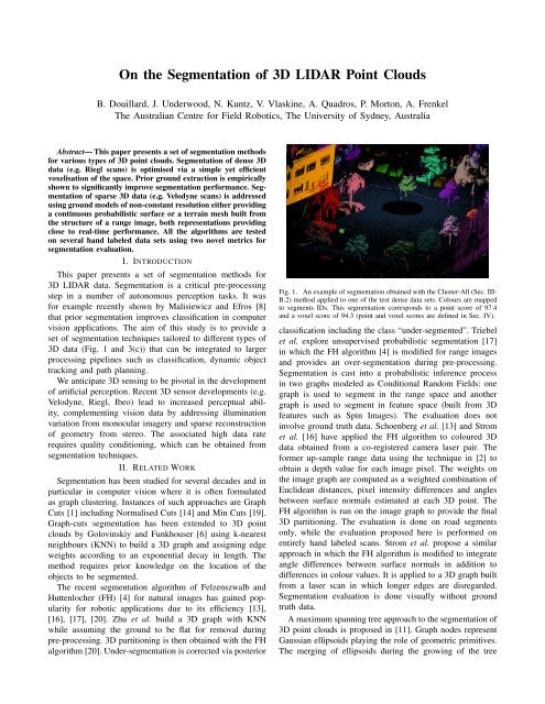
3D data (Fig. 1 and 3(c)) that can be integrated to larger
processing pipelines such as classification, dynamic object
tracking and path planning.
We anticipate 3D sensing to be pivotal in the development
of artificial perception. Recent 3D sensor developments (e.g.
Velodyne, Riegl, Ibeo) lead to increased perceptual ability,
complementing vision data by addressing illumination
variation from monocular imagery and sparse reconstruction
of geometry from stereo. The associated high data rate
requires quality conditioning, which can be obtained from
segmentation techniques.
II. RELATED WORK
Segmentation has been studied for several decades and in
particular in computer vision where it is often formulated
as graph clustering. Instances of such approaches are Graph
Cuts [1] including Normalised Cuts [14] and Min Cuts [19].
Graph-cuts segmentation has been extended to 3D point
clouds by Golovinskiy and Funkhouser [6] using k-nearest
neighbours (KNN) to build a 3D graph and assigning edge
weights according to an exponential decay in length. The
method requires prior knowledge on the location of the
objects to be segmented.
The recent segmentation algorithm of Felzenszwalb and
Huttenlocher (FH) [4] for natural images has gained popularity
for robotic applications due to its efficiency [13],
[16], [17], [20]. Zhu et al. build a 3D graph with KNN
while assuming the ground to be flat for removal during
pre-processing. 3D partitioning is then obtained with the FH
algorithm [20]. Under-segmentation is corrected via posterior
Fig. 1. An example of segmentation obtained with the Cluster-All (Sec. III-
B.2) method applied to one of the test dense data sets. Colours are mapped
to segments IDs. This segmentation corresponds to a point score of 97.4
and a voxel score of 94.3 (point and voxel scores are defined in Sec. IV).
classification including the class “under-segmented”. Triebel
et al. explore unsupervised probabilistic segmentation [17]
in which the FH algorithm [4] is modified for range images
and provides an over-segmentation during pre-processing.
Segmentation is cast into a probabilistic inference process
in two graphs modeled as Conditional Random Fields: one
graph is used to segment in the range space and another
graph is used to segment in feature space (built from 3D
features such as Spin Images). The evaluation does not
involve ground truth data. Schoenberg et al. [13] and Strom
et al. [16] have applied the FH algorithm to coloured 3D
data obtained from a co-registered camera laser pair. The
former up-sample range data using the technique in [2] to
obtain a depth value for each image pixel. The weights on
the image graph are computed as a weighted combination of
Euclidean distances, pixel intensity differences and angles
between surface normals estimated at each 3D point. The
FH algorithm is run on the image graph to provide the final
3D partitioning. The evaluation is done on road segments
only, while the evaluation proposed here is performed on
entirely hand labeled scans. Strom et al. propose a similar
approach in which the FH algorithm is modified to integrate
angle differences between surface normals in addition to
differences in colour values. It is applied to a 3D graph built
from a laser scan in which longer edges are disregarded.
Segmentation evaluation is done visually without ground
truth data.
A maximum spanning tree approach to the segmentation of
3D point clouds is proposed in [11]. Graph nodes represent
Gaussian ellipsoids playing the role of geometric primitives.
The merging of ellipsoids during the growing of the tree

is based on one of the two distance metrics proposed by
the authors, each producing a different segmentation “style”.
The resulting segmentation is similar to a super voxel type
of partitioning (by analogy to super pixels in vision) with
voxels of ellipsoidal shapes and various sizes.
Various methods focus on explicitly modeling the notion
of surface discontinuity. Melkumyan defines discontinuities
based on acute angles and longer links in a 3D mesh built
from range data [9]. Moosman et al. use the notion of convexity
in a terrain mesh as a separator between objects [10].
The latter approach is compared to the proposed algorithms
in Sec. V-B.
The contribution of this work is multi-fold: a set of segmentation
algorithms are proposed for various data densities,
which neither assume the ground to be flat nor require a prior
knowledge of the location of the objects to be segmented.
The ground is explicitly identified using various techniques
depending on the data type and used as a separator. Some of
the proposed techniques are close to real-time and capable
of processing any source of 3D data (Sec. III-C.1) or are
optimised by exploiting the structure of the scanning pattern
(Sec. III-C.2). All the methods are evaluated on hand labeled
data using two novel metrics for segmentation comparison
(Sec. V).
III. SEGMENTATION ALGORITHMS
A. Framework
This study considers the following three aspects of the segmentation
problem. First, it investigates various types of 3D
data: from dense (3D scans from a Riegl sensor for instance)
to sparse (single Velodyne scans). Second, different types of
model are used to represent and segment the ground. Three
main types of ground models are explored: grid based (as in
standard elevation maps [15], Sec. III-B), Gaussian Process
based (Sec. III-C.1) and mesh based (Sec. III-C.2). Third,
several types of 3D clustering techniques are tested and in
particular 3D grid based segmentation with various cluster
connectivity criteria is evaluated. The resulting algorithms
are compositions of a ground model and a 3D clustering
method. This study evaluates which algorithm provides better
segmentation performance for each data type.
The notions of dense and sparse data are here defined
based on a discretisation of the world with a constant
resolution. A data set will be considered to be dense if the
connectivity of most scanned surfaces can be captured with
the connectivity of non-empty cells (cells receiving at least
one data point). With sparser data, the number of empty cells
increases which causes objects to be over-segmented. The
algorithms proposed to segment dense data involve constant
resolution grid-based models, while the algorithms proposed
to process sparse data use ground representations which are
of non-constant granularity and implement various types of
interpolation mechanism as a way to bridge the holes in the
data.
B. Segmentation for Dense Data
The general approach used for dense data is a voxel grid
based segmentation. A three dimensional cubic voxel grid
is populated with 3D points and features are computed in
each voxel. Features include 3D means and variances as well
as density. This voxel grid approach is chosen due to its
simplicity, ease of representation both visually and in data
structures, and its ability to be scaled by adjusting voxel size
to insure usable density of data in the voxels.
For dense data segmentation four different variations on
this method are used, three of which have two stages and
one which is single stage. The extra stage in the two stage
processes is the determination of the ground partition, the
common stage is a 3D clustering process. For all methods,
voxels must meet minimum density requirements to be
considered for segmentation.
1) Ground Segmentation: The ground partition is found
by clustering together adjacent voxels based on vertical
means and variances. If the difference between means is less
than a given threshold, and the difference between variances
is less than a separate threshold, the voxels are grouped.
The largest partition found by this method is chosen as the
ground.
2) Cluster-All Method: Ground segmentation is performed
and the remaining non-ground points are partitioned
by local voxel adjacency only. The size of the local neighbourhood
is the only parameter. The ground is therefore
operating as a separator between the partitions. The general
outline of this method is shown in Algorithm 1. An example
of segmentation it produces is shown in Fig. 1.
Input : pCloud
Output : ground, voxelclusters
Parameters: res, method
1 voxelgrid ← FillVoxelGrid(pCloud,res) ;
2 ground ← ExtractGround(voxelgrid) ;
3 voxelgrid ← ResetVoxels(voxelgrid, ground) ;
4 voxelclusters ← SegmentVoxelGrid(voxelgrid,method) ;
Algorithm 1: The Dense Data Segmentation Pipeline, With Ground
Extraction
3) Base-Of Method: In order to test the benefit of using
the ground as a separator between objects, a technique which
does not rely of the extraction of a ground surface is also
defined. The algorithm considers voxels to be either flat
or non-flat depending on vertical variance. Flat voxels are
grouped together, as are non-flat voxels. Dissimilar voxels
are grouped only if the non-flat voxel is below the flat voxel.
This last criteria is based on the idea that sections of an object
are generally stacked on top of one another because of the
influence of gravity, hence some voxels are the base of other
voxels from the ground up. A typical example observed in
the data is the roof of a car, which may be disconnected
from to the rest of the car’s body without the ‘base-of’
relationship. In this case, flat voxels forming the roof of the
car are connected and non-flat voxels forming the body of the
car are also connected, resulting in two partitions. Applying
the base-of relationship, the body of the car is interpreted as
the base of its roof and the full car is connected into a single
segment.
4) Base-Of With Ground Method: Ground segmentation
is performed and then the Base-Of method is applied to the
remaining non-ground voxels.

C. Segmentation for Sparse Data
Two complementary segmentation methods for sparse data
are presented; Gaussian Process Incremental Sample Consensus
(GP-INSAC) and Mesh Based Segmentation. These
methods provide a sparse version of ExtractGround,
followed by the use of the Cluster-All approach from Section
III-B. The GP-INSAC method is designed to operate on
arbitrary 3D point clouds in a common cartesian reference
frame. This provides the flexibility to process any source of
3D data, including multiple 3D data sources that have been
fused in a common frame. By leveraging the sensor scanning
pattern, the Mesh Based method is optimised for 3D point
cloud data in a single sensor frame. This provides additional
speed or accuracy for particular sensor types.
1) Gaussian Process Incremental Sample Consensus (GP-
INSAC): The Gaussian Process Incremental Sample Consensus
(GP-INSAC) algorithm is an iterative approach to probabilistic,
continuous ground surface estimation, for sparse 3D
data sets that are cluttered by non-ground objects. The use of
Gaussian Process (GP) methods to model sparse terrain data
was explored in [18]. These methods have three properties
that are useful for segmentation: (1) they operate on sparse
data, (2) they are probabilistic, so decision boundaries for
segmentation can be specified rigorously, (3) they are continuous,
avoiding some of the grid constraints in the dense
methods. However, GP methods typically assume that most
of the data pertain to the terrain surface and not to objects
or clutter; i.e. they assume there are few outliers. Here,
the problem is re-formulated as one of model based outlier
rejection, where inliers are points that belong to the ground
surface and outliers belong to cluttered non-surface objects,
that will ultimately be segmented. The GP-INSAC algorithm
maintains the properties of GP terrain modeling techniques
and endows them with an outlier rejection capability.
A common approach to outlier rejection is the Random
Sample Consensus (RANSAC) algorithm [5], [12]. As the
complexity of the model increases, so does the number
of hypothetical inliers required to specify it, causing the
computational performance of RANSAC to decrease. For
complex models including GPs, an alternate approach is
presented, called Incremental Sample Consensus. Although
motivated by the cases where RANSAC is not practical,
INSAC is not a variant of RANSAC as in [12]. Deterministic
iterations are performed to progressively fit the model from
a single seed of high probability inliers, rather than iterating
solutions over randomly selected seeds.
The INSAC method is specified by Algorithm 2. Starting
with a set of data and an a-priori seed subset of high
confidence inliers, the INSAC algorithm fits a model to
the seed, then evaluates this for the remaining data points
(similar to the first iteration of RANSAC). All of the noninlier
points are compared with this model (using Eval from
Algorithm 2). INSAC uses probabilistic models that estimate
the uncertainty of their predictions, leading to two thresholds:
t model specifies how certain the model must be for in/outlier
determination to proceed. Subsequently, t data specifies the
Input : data, modelT ype, i seed
Output : i, o, u, model
Parameters: t data , t model
1 i = o = u = {};
2 i new = i seed ;
3 while size(i new) > 0 do
4 i = i ∪ i new;
5 model = Fit(modelT ype, i);
6 test = data − i;
7 {i new, o new, u new} = Eval (model, test, t data , t model );
8 o = o ∪ o new;
9 u = u ∪ u new;
10 end
Algorithm 2: The Incremental Sample Consensus (INSAC) Algorithm.
For brevity, i,o,u and t represent inliers, outliers, unknown and
threshold respectively.
normalised proximity of a datum (x) to the model prediction
(µ model ), required for the datum to be considered an inlier.
This is done using a variant of the Mahalanobis distance to
normalise the measure, given estimates of the noise in the
data and in the model (σ data , σ model , respectively). The two
rules are expressed by:
σ model < t model
and
x − µ model
√ < t data (1)
σ
2 x + σmodel
2
If the first inequality fails, a point is classified unknown.
Points that pass the first inequality are classified inliers if they
also pass the second inequality, otherwise they are outliers.
Starting from the seed, inliers are accumulated per iteration.
This allows INSAC to ’search’ the data to find inliers,
without allowing unknown points to corrupt the model.
Iterations are performed until no more inliers are found. The
process combines both extrapolation and interpolation of the
model, but only in regions where the certainty is sufficiently
high. This can be seen in the sequence of iterations of GP-
INSAC in Figure 2. The first iteration extrapolates but misses
a point because the data uncertainty is too large. By the third
iteration, it has captured this point using interpolation, once
the model/data agreement is more likely. Like RANSAC,
this method can be used with any core model, however the
justification to do so is strongest for complex probabilistic
models such as GPs.
The customisation of the INSAC algorithm for terrain
estimation using GPs is given in Algorithm 3. The algorithm
comprises four key steps; data compression, seed calculation,
INSAC and data decompression. Figure 2 shows three
iterations of the basic algorithm for simulated 2D data, to
illustrate the process, not including compression.
Input : x = {x i , y i , z i }, i = [0, N];
Output : i, o, u, model
Parameters: t data , t model , GP, r, d, R s, B s
1 x gm = GridMeanCompress(x,r);
2 x dgm = Decimate(x gm,d);
3 s dgm = Seed(x dgm ,R s,B s);
4 {, , , gp dgm } = INSAC(GP , s dgm , t data , t model );
5 {i gm, o gm, u gm} =Eval(gp dgm , x gm, t data , t model );
6 {i, o, u} = GridMeanDecompress(x, i gm, o gm, u gm);
7 model = gp dgm ;
Algorithm 3: The Gaussian Process INSAC (GP-INSAC) Algorithm
for Terrain Estimation, with optional Data Compression. i,o,u and t
represent inliers, outliers, unknown and threshold respectively.
The ability of GP models to handle sparse data allows
an optional step of compressing the data, to decrease the

(a) (b) (c)
Fig. 2. The GP-INSAC method from Algorithm 3 is run on simulated 2D data. A ground seed is chosen manually, shown in green. The output after the
first iteration is shown in (a), after three iterations in (b) and the 16th and final iteration in (c)
computation time. Compression is performed in two stages
in lines 1 and 2 of Algorithm 3. The data are first assigned
to a fixed 3D grid structure with a constant cell size of r
metres. In each cell, the contents are represented by their 3D
mean. In the second stage, the data are decimated by keeping
1 in every d of the grid means. The first stage compresses
the data towards uniform density, avoiding grid quantisation
errors by calculating the means. The second stage allows
further compression, without requiring larger (less accurate)
cell sizes.
Once the optional compression is performed, an initial
seed of likely ground points is determined using the application
specific Seed function. For this study, the points
within a fixed radius R s of the sensor that are also below
the base height B s of the sensor are chosen (|x| < R s
and x z < B s ), assuming this region is locally uncluttered
by non-ground objects. INSAC is then performed as per
Algorithm 2, on the decimated grid means. This classifies
the decimated grid mean data into the three classes; inliers,
outliers or unknown and provides the GP model representing
the continuous ground surface according to the inliers.
The data are then decompressed in lines 5 and 6 of
Algorithm 3. The GP model (from the decimated means)
is used to classify all of the un-decimated means, using
the same function from the INSAC method in line 7 of
Algorithm 2 and Equation III-C.1. Finally, the class of the
grid means is applied to the full input data by cell correspondence,
using GridMeanDecompress. The output is the
full classification of the original data, as inliers (belonging
to the ground), outliers (belonging to an object) or unknown
(could not be classified with high certainty).
For sparse segmentation, the ground data produced
by GP-INSAC in Algorithm 3 are considered as one
partition. The non-ground data are then processed by
SegmentVoxelGrid with the Cluster-All method from
Section III-B.2 to produce the remaining non-ground partitions.
Unknown points remain classified as such.
In Section V, the performance of the algorithm is demonstrated
with different parameter values and optimal parameter
choices are given by comparison with hand partitioned data.
2) Mesh Based Segmentation: The Mesh Based Segmentation
algorithm involves three main steps: (1) construction
of a terrain mesh from a range image; (2) extraction of the
ground points based on the computation of a gradient field
in the terrain mesh; (3) clustering of the non-ground points
using the Cluster-All method.
The generation of a mesh from a range image follows the
approach in [10], which exploits the raster scan arrangement
for fast topology definition (around 10 ms per scan). An
example of the resulting mesh is shown in Fig. 3(a). With
sparse data, such a mesh creates a point-to-point connectivity
which could not be captured with a constant resolution grid.
As a consequence the ground partition can be grown from
a seed region (here, the origin of the scan) through the
connected topology.
Once the terrain mesh is built, the segmenter extracts
the ground (function ExtractGround in algorithm 1) by
computing a gradient field in the mesh. For each node (i.e.
laser return), the gradient of every incoming edge is first
evaluated. The gradient value for the node is chosen as the
one with the maximum norm. The four links around a given
node are identified as: {UP, DOWN, LEFT, RIGHT}, with
DOWN pointing toward the origin of the scan. To compute
the gradient on the DOWN edge, for instance, the algorithm
traverses the mesh from one node to the following in the
DOWN direction until a distance of mingraddist is covered.
The gradient is then obtained as the absolute difference of the
height of the starting and ending node divided by the distance
between them. If a mingraddist length is not covered in
a given direction, the gradient is disregarded. Enforcing a
minimum gradient support length allows noise to be averaged
out: as can be seen in Fig. 3(a), the nodes nearer to the centre
of the scan are nearer to each other, which generates noisy
gradient estimates if consecutive nodes are used to calculate
the gradients (since the noise in their height values is of the
same magnitude as the length of the links connecting them).
Once the gradient field is computed, the ground partition
is obtained by growing a cluster of ground nodes from the
closest to the furthest raster line. In the closest raster line
(the inner most ring in Fig. 3(a)), the label GROUND is
assigned to the longest sequence of nodes s g with gradients
below maxgrad. Additionally, sequences of nodes s i from
the inner ring with gradients below the threshold maxgrad
are also marked GROUND if, given that n i and n g are
the closest nodes in s i and s g , respectively, their height
is within maxdh. For the other raster lines, a node is
marked as GROUND if its gradient value is below maxgrad,
and it has at least one of its direct neighbours already
identified as GROUND; whether this neighbour is in the
same raster line or in the previous one. This last requirement
encodes the iterative growing of the ground partition and
avoids non-ground flat partitions (such as the roof of a
car) to be mistaken as part of the ground. This propagation
process assumes that the ground can be observed around the
sensor; more specifically, it assumes that at least part of the
raster line nearest the sensor falls on the ground, and the
corresponding set of nodes form the longest flat sequence.
The propagation of the GROUND label is performed in both

(a) (b) (c)
Fig. 3. (a) The mesh built from the range image; points (nodes) identified as belonging to the ground are in white; other colours indicate off the ground
segments. (b) An example of transition detection around a car in the terrain mesh: ground points are in blue, non ground points in green, and transition
points in red. (c) An example of full segmentation obtained with the combination {Mesh Based segmenter, Cluster-All}. One colour corresponds to one
segment.
directions in each scan line (i.e. each scan line is traversed
twice) since intercepting objects may stop the propagation.
The extraction of the ground is illustrated in Fig. 3(c).
The last step in the extraction of the ground is the
identification of the transitions between the ground and the
objects above. The need for transition detection is developed
in [3] (Fig. 5). Its effect is illustrated in Fig. 3(b). Transitions
are detected by maintaining a buffer of consecutive
GROUND node heights (up to ten values are buffered in our
implementation). This buffer is slid along each raster line
first, and then along each radial line, while GROUND node
heights are added in a First In First Out fashion. The buffer
is emptied when starting the processing of the next line. A
node is marked as TRANSITION if it does not belong to the
ground based on its gradient but its height is within maxdh
of the buffer mean height. The buffer is slid twice on each
scan and radial line; once in each direction along the line in
order to identify the transitions on all sides of an object. As
illustrated in Fig. 3(b), transition detection allows a tighter
segmentation of objects which is essential in cluttered areas.
Once the ground is extracted, the NON-GROUND points
are fed to a voxel grid and a Cluster-All segmentation is
applied. Note that the points identified as TRANSITION are
not passed to the 3D segmenter since this allows a tighter
segmentation of objects. This completes the segmentation
process as implemented by the Mesh Based Segmenter.
Its output is illustrated in Fig. 3(c). In the experiments
(Sec. V-B), the three parameters mingraddist, maxdh and
maxgrad are optimised based on hand-labeled segmentations.
IV. METRIC FOR SEGMENTATION EVALUATION
A metric is proposed to quantify the agreement between
two segmentations of the same set of data. This can be
used to quantify the performance of different segmentation
algorithms, by comparison to a hand segmented scene. The
general concept of the metric is illustrated in Fig. 4. The tree
marked B is the manual segmentation and the tree marked A
is an example of flawed segmentation. The largest segment
of the voxels in A that comprises the tree is considered the
match, in this case the red area of the tree top, and all other
partitions are considered errors. Once a segment has been
considered as a match, it will be considered as an error in
any subsequent match attempts.
The specific comparison process is as follows. First the
partitions of the hand-picked data are sorted from largest
Fig. 4.
Example of Segmentation Comparison
to smallest. For each reference partition, each data point is
matched to the same point in the test segmentation. A list of
partition sizes is accumulated based on the partition IDs of
the points. The largest partition of test points that correspond
to the given hand-picked partition is then considered to be a
match. The partition ID that is considered matching is then
marked as used and then when any other points with that
ID are found they are considered to be in error. Because the
comparison is performed in order from the largest partition
to the smallest, if a small object is incorrectly grouped to
a large object, the smaller object will be considered to be
erroneously partitioned and not the larger object. From the
points marked as matches and those marked as errors, a
percentage match is calculated.
Alternative metrics are also considered. In particular, scoring
in terms of voxels instead of points. Since all points in a
voxel must have the same partition ID, voxels can be marked
as matched or errors when the status of any point within
the voxel is determined. Then the voxel match percentage
is also calculated. The voxel match percentage tends to be
more volatile than the point match percentage. The quality
of partitioning of smaller, sparser, more difficult to partition
objects is usually better represented by the voxel score due
to less domination by ground and wall points. For example,
in one of the data sets used here, the ground comprises
over 700,000 points of the 1.6 million points in the scan
(44%), but only 35,600 voxels of the 143,000 voxels in the
segmentation (24%).
V. EXPERIMENTS
This empirical analysis follows the principles laid out
by Hoover et al. in their reference work on experimental
evaluations of segmentation methods for range images [7]. In
particular, the parameter space of each algorithm is uniformly
sampled to find the combination of parameters providing
the best segmentation results with respect to several hand
labeled data sets (the use of more sophisticated optimisers
is left for future work). Match percentages (relative to the
hand segmented data) and computation times are recorded
and averaged over the test data sets for each combination

of parameters tested. The best results for dense and sparse
data are provided in Tables I and II, respectively. The best
results across methods are indicated in bold. The type of
implementation used is also indicated. The output of each
technique is further illustrated in the video associated with
this submission (a longer version of this video is available at:
http://www.acfr.usyd.edu.au/afmr/segmentation/icra11results.wmv).
A. Dense Data Results
Four hand labeled data sets (with point-wise labels) are
used in this first set of experiments: two are formed from a
single Riegl scan, one acquired at Drexel University, US,
and a second one at the University of Sydney, Australia
(Fig. 1); another set is generated by combining vertical
scans from a SICK laser with the navigation solution of the
mobile platform the sensor is mounted on; and a fourth set is
obtained by combining Velodyne scans and navigation data.
The four point clouds were acquired in static environments.
1) Cluster-All Segmentation Method: For this experiment,
the role of voxels size was tested. The two plots in Fig. 5 are
the point and voxel scores versus voxel size in centimeters
and neighbourhood. The neighbourhood value is the absolute
magnitude of the distance two voxels can be away from each
other, in terms of voxel grid spaces. For example two voxels
that are touching but one grid off in x or y would have a
magnitude of 1, and if the voxels were only touching corner
to corner that would be a magnitude of 3. The voxel size
tests show a peak at 0.2m. In terms of computation times,
at a voxel sizes of 0.1m, 0.2m, and 0.4m processing took
on average 8.02s, 4.30s, and 3.82s respectively (these times
cannot be directly compared to the other tests because a
different data structure was used to allow a larger number of
voxels to be represented). The peak match percentage occurs
with a voxel size of 0.2m. Since a significant time penalty
is incurred for smaller voxels and minimal time savings are
achieved with larger voxels, the conclusion can be made that
0.2m is optimal based on these tests. The scores reported in
Table I correspond to this parameter choice.
Fig. 5. Cluster-All Segmentation, Scores of Variance Tests and Voxel Size
Tests.
A variant of Cluster-All involving a varying neighbourhood
size was also tested. It is illustrated in Fig. 7(a). The
density of objects and the density of scan points is greater at
lower heights above ground due to objects naturally resting
on the ground and the corresponding proximity of the sensor.
Employing larger neighbourhoods a certain distance above
the ground can prevent over-segmentation of high sparse
objects while not risking under-segmentation of objects close
together on the ground. The corresponding results are reported
in the line ‘Cluster-All with Variable Neighbourhood’
Fig. 6. Base-Of Segmentation, Match Results vs Standard Deviation and
3D Neighbourhood.
of table I. In these tests the neighbourhood was restricted to 3
for voxels less than 2 meters above the ground and extended
to 6 otherwise.
2) Base-Of Segmentation Method: For this method two
parameters were varied and all tests were run both with
and without the ExtractGround operation (Algorithm 1).
Fig. 6 shows 3D plots of the average results for the four
dense data sets. While Base-Of without ground extraction
has the advantage of being almost twice as fast as the ground
based methods, it is behind the other techniques in terms of
accuracy. This result experimentally confirms the usefulness
of explicit ground extraction in 3D segmentation.
B. Sparse Data Results
Four hand labeled Velodyne scans (with point-wise labels)
are used for the evaluation of the sparse methods. The results
are presented in Table II and were obtained by averaging
performance and computation times over the four labeled
scans (the same as the dense data results).
1) Cluster-All Segmentation: The following three parameters
are varied to obtain the best point and voxel scores:
maxvstd, the maximal vertical standard deviation in a voxel
below which this voxel is identified as belonging to the
ground in the function ExtractGround; groundres, the
resolution of the grid used in ExtractGround; objectres,
the resolution of the grid used in SegmentVoxelGrid.
The results are shown in Fig. 7(b). In both cases, the
optimal parameter values are 0.3m for maxvstd, 0.5m for
groundres and 0.2m for objectres, and correspond to the
best scores reported in Table II.
2) GP-INSAC Segmentation: The complete GP-INSAC
sparse segmentation method has a total of seven parameters,
grouped by the stages in the pipeline. INSAC requires t data
and t model , the cylindrical seed region requires R s and B s ,
data compression uses r and d, and the final partitioning
step is parameterised by the grid resolution. The GP model
employs a squared exponential covariance with three parameters:
length scale, process and data noise (ls, σ p , σ d ), which
are learnt off-line with a maximum likelihood approach [18],
by manually providing segments of ground data. Once learnt,
these parameters are fixed for the GP-INSAC algorithm.

TABLE I DENSE SEGMENTATION MATCH RESULTS
Method Point Score Range Voxel Score Range Computation Times
Cluster-All 97.4 94.3 1.60 - 1.47 sec (C++)
Cluster-All with Variable Neighbourhood 97.7 94.9 1.71 - 1.36 sec (C++)
Base-Of 88.5 79.8 0.76 - 0.70 sec (C++)
Base-Of With Ground 97.2 93.9 1.56 - 1.38 sec (C++)
TABLE II SPARSE SEGMENTATION MATCH RESULTS
Method Point Score Range Voxel Score Range Computation Times
Cluster-All 0.81 0.71 0.42 - 0.42 sec (C++)
GPINSAC 0.89 (on 96%) 0.83 0.17 sec (C++)
Mesh Based 0.92 0.88 0.27 - 0.29 sec (C++)
Convexity Based Segmentation [10] 0.71 0.63 1.76 - 1.69 sec (Python/C++)
(a) (b) (c)
Fig. 7. (a) Segmentation with Fixed Neighbourhood (A) and Variable Neighbourhood (B) showing better segmentation with use of a variable neighbourhood.
(b) Point scores (left) and voxel scores (right) obtained when varying the three parameters maxvstd, groundres and objectres in the Cluster-All algorithm.
Colours are mapped to scores. The optimum is indicated in each figure by a larger red dot. For the point score, the range of values is: 0.38 to 0.81; for the
voxel score, it is: 0.24 to 0.71. (c) Same colour coding as in (b) for the parameters mingraddist, maxdh and maxgrad of the Mesh Based Segmenter.
For the point score, the range of values is: 0.56 to 0.92; for the voxel score, it is: 0.47 to 0.88.
The algorithm was run on a range of parameters.
The seed cylinder was measured and fixed to {R s =8m,
B s =−1.6m} and the optimal partition resolution for
SegmentVoxelGrid was fixed to 0.2m, as determined
in Section III-B. Six sets of the three GP parameters were
learnt, from the four test scans and from two other training
scans. The additional two were included to allow a separate
source of training data to be used, allowing the algorithm to
be tested on independent test data.
The algorithm was evaluated with the segmentation metric
from Section IV and timed on a 2GHZ dual core PC.
The results are shown in Figure 8. The parameter sets that
produced results with a point score above 80%, a percent
classified > 90% and processing time < 0.25s were selected.
The individual parameters that most frequently led to this
selection were chosen as optimal. As such, they are likely
to be the most stable. This corresponds to the parameter
set Compression{r=0.6m, d=30}, INSAC{t model =0.2m,
t data =3sd}, GP {ls=14.01m, σ p =0.88m, σ d =0.060m}. Interestingly,
the optimal GP parameters were learnt from one
of the two separate training samples.
The results using the optimal parameter choice from this
test are shown in Table II. The metric indicates an accurate
segmentation is produced in the fastest computation time.
However, parameters could be chosen to further emphasise
accuracy for a larger computational cost. Future work includes
testing the algorithms for stability on a larger set
of data and it is suspected that GP-INSAC will require a
’slower’ parametrisation to achieve long term stability. In
that case, the mesh segmentation is likely to be closer to real
time performance when processing can be done in the sensor
frame. The key differentiator of the GP-INSAC algorithm is
that it can process arbitrary 3D data from any source or
multiple fused sources.
3) Mesh Based Segmentation: The following three parameters
are varied to obtain the best point and voxel scores:
mingraddist, maxgrad, and maxdh (detailed in Sec. III-
C.2). The test results are shown in Fig. 7(c). The best point
score is achieved when mingraddist is 0.4m, maxgrad is
0.1 and maxdh is 0.05m. The best voxel score is achieved
when mingraddist is 0.35m, maxgrad is 0.1 and maxdz
is 0.1m. The corresponding scores are reported in Table II.
Based on the results in Sec. V-B.1, the resolution of the grid
used in SegmentVoxelGrid was set to 0.2m.
By generating a mesh of varying resolution in the sensor
frame as opposed to relying on a fixed resolution grid
for ground model as in the Cluster-All method, the Mesh
Based Segmenter is able to better recover the underlying
connectivity of objects. Table II shows an improvement in
voxel score of up to 24%. Directly representing the sparsity
of the data also allows to reduce the size of the data structures
deployed which in turn leads to gain in computation times.
Table II shows that the Mesh Based Segmenter is about 30%
faster than the ‘Cluster-All’ method (both implementations
are run on a 3GHz desktop computer). The tendency would
be reverted however in the case of dense data since the terrain
mesh would become denser while a fixed size grid effectively
sparsifies the data to an amount related to its resolution.
4) Convexity Based Segmentation: The method proposed
by Moosmann et al. [10] was implemented and tested for
this analysis since the Mesh Based Segmenter relies on the
same terrain mesh. The main differences between the two
approaches are related to the identification of the ground.

1
0.95
0.9
0.95
0.9
0.89
0.9
0.85
0.88
X: 0.1716
Y: 0.8891
Mean Fraction Classified (%)
0.85
0.8
0.75
0.7
0.65
Mean Point Score (%)
0.8
0.75
0.7
0.65
Mean Point Score (%)
0.87
0.86
0.85
0.84
0.83
0.6
0.6
0.82
0.55
0.55
0.81
0.5
0.4 0.5 0.6 0.7 0.8 0.9 1
Mean Point Score (%)
0.5
0 1 2 3 4 5 6
Mean Time (s)
0.8
0.16 0.18 0.2 0.22 0.24 0.26
Mean Time (s)
(a)
(b)
(c)
Fig. 8. The results of the GP-INSAC method from Algorithm 3 for different parameter choices, averaged over the four test Velodyne scans. The trade-off
between the percentage of points classified vs point score is shown in (a), which indicates a near complete and accurate classification is possible. In (b)
the point score and processing time is compared. In (c), only the results with a point score > 0.8, a percent classified > 0.9 and processing time < 0.25s
seconds are shown. The result from the optimal parameters is highlighted.
Here it is integrated into to the segmentation process, while
in [10] it is obtained from posterior classification . Also, the
reasoning in the mesh is used here for ground extraction only
(in the function ExtractGround) while it generates the
segmentation of the entire 3D space in [10]. Table II shows
that the performance of the latter method is lower. As for the
other techniques, a range of parameter values was tested and
results averaged over the four labeled scans. Following the
notations in [10], ɛ 1 was varied from 0 to 45 with a step size
of 5, ɛ 2 was varied from 0 to 60 with a step size of 10, and
ɛ 3 from 0 to 0.7 with a step size of 0.1. For both point and
voxel scores, the optimal values were found to be 40 for ɛ 1 ,
50 for ɛ 2 and 0.5 for ɛ 3 . The lower performance is in part due
to the limited size of the labeled set and the behaviour of the
segmentation metric: for certain combinations of parameters,
the segmentation is visually close to the one obtained with
the mesh segmenter but the ground is divided into a few main
parts which causes a large penalty, since the ground has a
dominating weight in both the point and the voxel scores.
VI. CONCLUSION
This study has proposed a set of segmentation methods
designed for various densities of 3D point clouds. It first provided
empirical evidence of the benefit of ground extraction
prior to object segmentation in the context of dense data. The
Cluster-All method has achieved the best trade off in terms
of simplicity, accuracy and computation times. Its limitations
were shown in the context of sparse data and two novels
segmentation techniques were proposed for the latter case:
the GP-INSAC algorithm for probabilistic ground modeling
and for the processing of any 3D point cloud sparse or dense,
potentially formed of data accumulated from several sensors;
a Mesh Based technique, optimised for the processing of
range images. All the algorithms were evaluated on several
sets of hand labeled data using two novel metrics.
REFERENCES
[1] Y. Boykov and G. Funka-Lea. Graph cuts and efficient nd image
segmentation. International Journal of Computer Vision, 70(2):109–
131, 2006.
[2] J. Diebel and S. Thrun. An application of markov random fields to
range sensing. Advances in neural information processing systems,
18:291, 2006.
[3] B. Douillard, J. Underwood, N. Melkumyan, S. Singh, S. Vasudevan,
C. Brunner, and A. Quadros. Hybrid elevation maps: 3d surface models
for segmentation. In Proc. of the IEEE/RSJ International Conference
on Intelligent Robots and Systems (IROS), 2010.
[4] P.F. Felzenszwalb and D.P. Huttenlocher. Efficient graph-based image
segmentation. International Journal of Computer Vision, 59(2):167–
181, 2004.
[5] Martin A. Fischler and Robert C. Bolles. Random sample consensus:
a paradigm for model fitting with applications to image analysis and
automated cartography. Commun. ACM, 24(6):381–395, 1981.
[6] A. Golovinskiy and T. Funkhouser. Min-cut based segmentation of
point clouds. princeton University.
[7] A. Hoover, G. Jean-Baptiste, X. Jiang, P.J. Flynn, H. Bunke, D.B.
Goldgof, K. Bowyer, D.W. Eggert, A. Fitzgibbon, and R.B. Fisher.
An experimental comparison of range image segmentation algorithms.
IEEE transactions on pattern analysis and machine intelligence,
18(7):673–689, 1996.
[8] T. Malisiewicz and A. Efros. Improving spatial support for objects via
multiple segmentations. In British Machine Vision Conference, pages
282–289, 2007.
[9] N. Melkumyan. Surface-based Synthesis of 3D Maps for outdoor Unstructured
Environments. PhD thesis, University of Sydney, Australian
Centre for Field Robotics, 2008.
[10] F. Moosmann, O. Pink, and C. Stiller. Segmentation of 3D Lidar Data
in non-flat Urban Environments using a Local Convexity Criterion. In
IEEE Intelligent Vehicles Symposium, pages 215–220, 2009.
[11] F. Pauling, M. Bosse, and R. Zlot. Automatic Segmentation of 3D
Laser Point Clouds by Ellipsoidal Region Growing. In Proc. of the
Australasian Conference on Robotics & Automation (ACRA), 2009.
[12] Rahul Raguram, Jan-Michael Frahm, and Marc Pollefeys. A comparative
analysis of ransac techniques leading to adaptive real-time
random sample consensus. In David Forsyth, Philip Torr, and Andrew
Zisserman, editors, Computer Vision ECCV 2008, volume 5303 of
Lecture Notes in Computer Science, pages 500–513. Springer Berlin
/ Heidelberg, 2008.
[13] J. Schoenberg, A. Nathan, and M. Campbell. Segmentation of dense
range information in complex urban scenes. In Proc. of the IEEE/RSJ
International Conference on Intelligent Robots and Systems (IROS),
2010. To appear.
[14] J. Shi and J. Malik. Normalized cuts and image segmentation. IEEE
Transactions on pattern analysis and machine intelligence, 22(8):888–
905, 2000.
[15] B. Siciliano and O. Khatib. Springer handbook of robotics. Springer,
2008.
[16] J. Strom, A. Richardson, and E. Olson. Graph-based segmentation of
colored 3d laser point clouds. In Proc. of the IEEE/RSJ International
Conference on Intelligent Robots and Systems (IROS), 2010. To appear.
[17] R. Triebel, J. Shin, and R. Siegwart. Segmentation and unsupervised
part-based discovery of repetitive objects. In Proceedings of Robotics:
Science and Systems, Zaragoza, Spain, June 2010.
[18] S. Vasudevan, F. Ramos, E Nettleton, and H. Durrant-Whyte. Gaussian
process modeling of large-scale terrain. Journal of Field Robotics,
26:812840, 2009.
[19] Z. Wu and R. Leahy. An optimal graph theoretic approach to
data clustering: Theory and its application to image segmentation.
IEEE transactions on pattern analysis and machine intelligence, pages
1101–1113, 1993.
[20] X. Zhu, H. Zhao, Y. Liu, Y. Zhao, and H. Zha. Segmentation and
classification of range image from an intelligent vehicle in urban
environment. In Proc. of the IEEE/RSJ International Conference on
Intelligent Robots and Systems (IROS), 2010. To appear.