Ch. 9 pt 1

Chapter 9: TESTS OF HYPOTHESES
FOR A SINGLE SAMPLE
Part 1: Intro to Hypothesis Testing
Sections 9-1, 9-2, 9-3
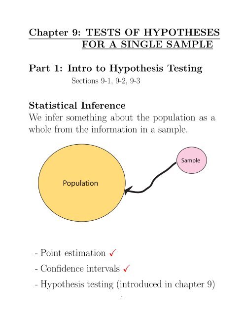
Statistical Inference
We infer something about the population as a
whole from the information in a sample.
Sample
Population
- Point estimation ̌
- Confidence intervals ̌
- Hypothesis testing (introduced in chapter 9)
1

Hypothesis Testing
Sections 9-1, 9-2, 9-3
We’ll start with an illustration...
• Example: Reduction of car emissions
A certain automobile engine emits 100 mg
of nitrogen oxides per second on average. A
modification to the engine has been proposed
that may reduce the emissions.
The new design will be put into production
IF it can be demonstrated that its mean emission
rate is less than 100 mg/s.
To make a decision, a random sample of
n = 50 modified engines is taken and
emission measurements are recorded.
2

The sample mean is ¯x = 92 mg/s and the
sample standard deviation is s = 21 mg/s.
A normal probability plot suggests emissions
follow a normal distribution.
Isn’t 92 far enough below 100 for us to say
the modified engine is better
Is there enough evidence to completely change
the manufacturing line and switch which
engine is produced
3

STATISTICAL QUESTION:
Could we have gotten this low of a sample
mean emission ¯x even if the modified engine
WASN’T any better than the first (i.e. it’s
population mean was actually 100)
Could we have grabbed a sample that happened
to have many low emission values eventhough
the population mean was 100
To make a decision on the engines, we want
to quantify the above question with a probability:
“Given that the true population mean emission
is 100 mg/s, what is the probability
of observing an emissions ¯x this low or
lower
4

Recall from the last chapter:
If we assume µ = 100 and n large, we have
¯X ∼ N(100, σ2
n ).
This is a known behavior of the sample mean.
Probability of interest:
Given µ = 100 (engine not any better),
P ( ¯X ≤ 92) =
Since σ 2 is unknown in this case, we have
T = ¯X − µ
S/ √ n ∼ t n−1
where S is the sample standard deviation
and T has a t distribution with n−1 degrees
of freedom (and n = 50 in this example).
5

P ( ¯X ≤ 92) = P
( ¯X − µ
S/ √ n
)
92 − 100
≤
21/ √ 50
= P (T ≤ −2.69)
because T ∼ t 49
t with 49 df
t(49) density
−3 −2 −1 0 1 2 3
T
= 0.0049
6

NOT VERY LIKELY...
The probability of observing an emissions ¯x
this low or lower, given that the true population
mean is 100 mg/s is
0.0049
This suggests that our initial assumption in
the calculation, that the true mean was 100,
is perhaps incorrect.
For this reason, we reject the assumption of
µ = 100 in favor of the ‘alternative’, that
the true mean emissions IS LESS THAN 100
mg/s.
We don’t know FOR SURE, but there’s strong
evidence against someone saying that the mean
of the modified engine is 100 mg/s.
7

If it was 100 mg/s, we would very rarely see
an ¯x this low (could happen, but not likely).
What’s unlikely enough to actually reject
the initial assumption (that the two engine
models were equal)
There’s some opinion here, but we often use
0.05 as a threshold. Anything less than this
is considered rather unlikely.
————————————————————
We have essentially just performed a hypothesis
test, now we will formalize the procedure...
8

• General set-up for testing a
hypothesis for µ
1. State your null H 0 and alternative H 1
hypotheses.
(The null is what we assume to be true.)
H 0 : µ = µ 0
(The subscript on µ 0 is used to emphasize
that this value is the assumed mean under
the null hypothesis being true.)
There are 3 choices for the alternative,
either...
* H 1 : µ ≠ µ 0 (two-sided alternative)
* H 1 : µ < µ 0 (one-sided alternative)
* H 1 : µ > µ 0 (one-sided alternative)
9

2. Calculate the test statistic (either a Z or T ).
(In this example, the test statistic was a
T , we’ll make a conclusion based on this.)
3. Compute the probability of observing a test
statistic this extreme, or more extreme,
under the null being true.
(This probability is called a p-value.)
4. State your conclusion with respect to the
problem:
Either...
‘Reject the null’
or
‘Fail to reject the null’.
5. Be sure to verify any assumptions that were
needed.
(This is usually a normal probability plot
for verifying normality which is needed to
have T ∼ t n−1 ).
10

• Example: Formalizing the emissions
hypothesis test
1. State your null H 0 and alternative H 1
hypotheses.
H 0 : µ = 100
H 1 : µ < 100
(this is a one-sided
hypothesis test with
µ 0 = 100)
2. Calculate the observed test statistic.
t 0 = ¯x − µ 0
s/ √ n
=
92 − 100
21/ √ 50 = −2.69
(The subscript on t 0 is used to emphasize
the fact that we’re assuming the mean to
be µ 0 .)
11

3. Compute the probability of observing a
test statistic this extreme, or more extreme,
under the null being true (i.e. compute the
p-value).
Under H 0 true, T 0 = ¯X−µ 0
S/ √ n ∼ t 49, and
P (T 0 ≤ −2.69) = 0.0049
t with 49 df
t(49) density
−3 −2 −1 0 1 2 3
Thus, because this is a one-sided hypothesis
test, the p-value=0.0049.
T
12

p-value=0.0049...
“If the true mean is really µ = 100, then
the probability of observing a sample mean
(from a sample of size n = 50) this far below
100 (or even farther) is only 0.0049.”
4. State your conclusion for the hypothesis
test:
Using 0.05 or
5
100
as a threshold for ‘unlikeliness’,
we have
p-value = 0.0049 < 0.05
and we reject the null in favor of the
alternative, which is that µ < 100.
13

5. Be sure to verify any assumptions that
were needed.
As stated earlier, we checked the normal
probability plot of the emission values and
it was OK, and the needed requirement for
T 0 ∼ t 49 (that the parent population was
normally distributed) was fulfilled.
When we reject H 0 , we say the test was significant.
For this example, we say there was significant
statistical evidence that the modified engine
has a mean emissions lower than 100 mg/s.
So, there was strong evidence that the modified
engine is better.
14

• Why do we use this test statistic T 0 to test
H 0 : µ = µ 0
T 0 = ¯X − µ 0
S/ √ n
Let’s pick-apart this statistic...
– Under H 0 true, E( ¯X) = µ 0 and the expected
value of the numerator in T 0 is 0,
and the distribution of T 0 is unimodal centered
at zero.
– If ¯X is far from µ0 in either direction, the
numerator in T 0 will be ‘large’(+ or −)
leading to a ‘large’ T 0 , leading to rejection
of H 0 .
A ‘large’ or ‘extreme’ T 0 would not be expected
if H 0 was true (we expect T 0 to
‘bounce-around ’ 0 if H 0 true).
15

– But what is a ‘large’ difference or ¯X −µ 0
This is where the denominator comes into
play. ‘Large’ is based on our sample size
and the variability in the population σ 2
(which shows up in S).
For one thing, scale matters. A ‘large’ difference
in ¯X −µ 0 on a nanoscale will probably
not be the same as a large difference
in kilometers (S will make this adjustment
here).
We also know that the expected squared
distance of ¯X from µ goes down as n increases.
This also has to be taken into
account for deciding what is ‘large’.
Bottom line... if we observe a realized t 0
value that is in the far tail of the T 0 distribution,
it suggests we should reject H 0 .
16

Some comments on terminology...
• The Null Hypothesis:
– It is what we assume to be true upon entering
the hypothesis test
In many formal arguments, we often assume
something to be true, and then see
if we can contradict this assumption
later.
We’re not looking to prove something
here, but we may find that the data were
not very likely to have occurred under the
null being true, which was the assumption
we made (in which case we reject the null).
– Often, the null is the less interesting statement
to the researcher.
17

– Innocent until proven guilty.
We’re being cautious, we’re giving the
status-quo the benefit of the doubt.
– The situation is assumed uninteresting
until evidence can show (beyond reasonable
doubt) that something interesting is
going on.
– Symbolized by H 0 .
– It is a statement about a population parameter,
not a statistic.
– Example: the modified engine data,
H 0 : µ = 100
18

• P-value:
– The p-value represents the probability of
obtaining a test statistic as extreme (or
more extreme) in magnitude than the observed
test statistic under H 0 true
– If you perform a two-sided hypothesis test
H 0 : µ = µ 0 vs. H 1 : µ ≠ µ 0 ,
the p-value is the probability in both tails
(example on slide p.23)
– Large test statistic (in absolute value) ⇔
small p-value
– Small p-values are evidence against the
null hypothesis (as are large test statistics)
– When we make a decision to reject H 0 it
is because the p-value is small
19

– A small p-value says we would have been
very unlikely to have gotten a sample with
data like this if H 0 were true
– The p-value is not the probability that H 0
is true
– We use the calculated p-value to make a
conclusion or decision on the hypothesis
test based on a chosen significance level α
(on next slide):
∗ Reject the null hypothesis
∗ Fail to reject the null hypothesis
(i.e. accept the null hypothesis)
– We do not prove the null hypothesis true,
this is not how things are set-up. We will
assume it to be true right from the start
of the procedure.
20

• The significance level α:
– How low must a p-value be to reject the
null
– We set a threshold that will control our
chance of making a particular mistake.
What mistake
REJECTING H 0 WHEN H 0 IS
ACTUALLY TRUE.
This is called a type I error.
This is often seen as a big mistake.
In the emissions example, the company
would completely re-do their engine manufacturing
set-up if they reject. This would
be a big waste if the modified engine actually
wasn’t any better.
21

– We set the chance of such a mistake to be
α which is often set at 0.05 (though 0.01
and others are also seen).
We simply accept a 5% chance that we
make a type I error. For most situations,
this chance of a mistake is considered low
enough.
– By only rejecting when the p-value is less
then α we control the type I error at the
α level.
α = P (type I error)
= P (reject H 0 when H 0 is true)
= P (reject H 0 |H 0 is true)
= P (a false positive occuring)
22

• Example: An example where σ 2 is known
or you have very large sample
If σ 2 is known, or you have a very large
sample, the test statistic will be the
Z test statistic, instead of the T .
An inspector measured the full volume of a
simple random sample of n = 100 cans of
juice that were labeled as containing 12 oz.
The sample had a mean volumed 11.98 oz
and a standard deviation of 0.19 oz.
Let µ represent the mean fill volume for all
cans of juice recently filled by the machine.
Perform a hypothesis test that µ = 12 versus
µ ≠ 12 at the α = 0.05 significance level.
23

ANS:
24