Split-plot design with covariate

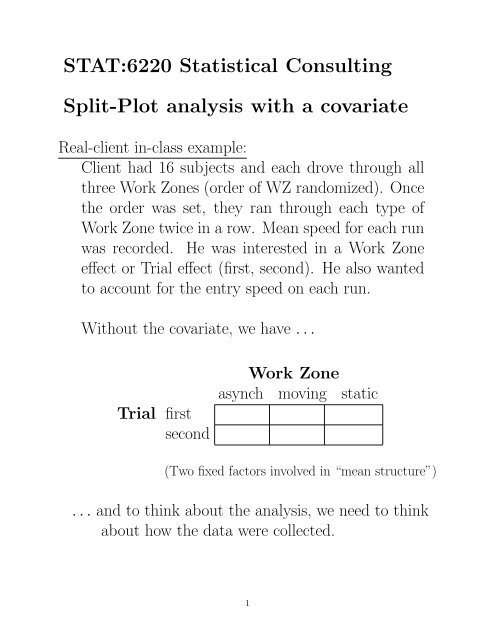
NOTE: If you saw the two runs within each Work Zoneas simply ‘subsampling’, and the multiple measurementswere essentially done to get a more precise measurementfor the driver in that Work Zone, then your model wouldlook different than the split-plot approach I’ve been describing.For instance, ‘trial’ would not be a fixed effect, but wewould instead have a random replicate effect nested ina Workzone*SUBJECT combination. Perhaps we couldcall this a ‘subsampled RCBD’ or ‘pseudoreplication’.The ANOVA table for RCBD with subsampling:Sourcedf EMSBLOCK15 σ 2 + 2σδ 2 + 2 ∗ 3σ2 ∑baj=1WorkZone 2 σ 2 + 2σδ 2 + 2 ∗ 16 α 2a−1BLOCK*WorkZone 30 σ 2 + 2σδ2REP(BLOCK*WorkZone) 48 σ 2c.total 95If subsampling is done, it is still the MS BLOCK∗W orkZonethat is used to test for a WorkZone effect.Because the two observations within a WZ werecollected over time, I (instead) felt that they heldinformation on a potential time effect.3

Chapter 7 Analysis of Covariance.Section 7.8 Example: Split-Plot Design withthe Covariate Measured on the Small−Size Experimental Unit or SubplotThe data are from a study designed by a researcherto evaluate the effectiveness of three teaching methods.Four teachers were trained in each method.The twelve teachers were randomly assigned to twelveclasses of eight students consisting of four males andfour females.The experimental unit for the teaching method isthe teacher (or class). Besides method, the researcherwas also interested in the possible differencein gender response to the three teaching methods.Thus, gender is the treatment for the small-size experimentalunit, the student.The covariate is the student’s IQ score.5

Full model with covariate to describe the test scores:(assumes linear relationship between IQ and response)Y ijkm = α ik + β ik x ijkm + t j(i) + ɛ ijkm (1)where t j(i) ∼ iid N(0, σ 2 t )ɛ ijkm ∼ iid N(0, σ 2 ɛ )α ik ≡ intercept of i th teaching method and k th gender.β ik ≡ slope of i th teaching method and k th gender.x ijkm ≡ IQ on student m in treatment combination iktaught by teacher j.t j(i) ≡ random teacher effect (nested in a method).Teaching Method1 2 3Gender malefemaleEach ‘cell’, specified by an (i, k) combination, is allowedto have it’s own regression line (i.e. slope and intercept).Authors describe the full model as having ‘factorial effects’for both intercepts and slopes.Correlation between observations is induced through theteacher effect.6

SAS code for full model:proc mixed data=ex_7_8;class teacher meth gend;model score=meth gend meth*gend iqiq*gend iq*methiq*gend*meth/ddfm=satterth residual;random teacher(meth);run;The error terms are no longer ‘clean’ like in the traditionalsplit-plot design. Using the ddfm=satterth allows forerror d.f. to be calculated as we saw in our design coursefor approximate F-tests.Type 3 Tests of Fixed EffectsNum DenEffect DF DF F Value Pr>Fmeth 2 83.4 0.41 0.6662gend 1 75.8 0.09 0.7693meth*gend 2 75.8 0.23 0.7971iq 1 76.4 148.76

After iterative removal of non-significant terms involvingIQ (in the mean structure), the final model allowed forparallel regression lines across the six cells.proc mixed data=ex_7_8;class teacher meth gend;model score=meth gendmeth*gend iq/ddfm=satterth residual;random teacher(meth);run;Type 3 Tests of Fixed EffectsNum DenEffect DF DF ∗ F Value Pr>Fmeth 2 9.03 10.05 0.0051gend 1 80 2.65 0.1074meth*gend 2 80 6.09 0.0034iq 1 81.3 158.52

The six intercepts may or may not be significantly different(i.e. some of the lines may not be significantly differentfrom each other).Contrasts could be used to compare lines, or one coulduse the SLICE option to easily request comparisons ofgender within each method (or comparisons of methodwithin each gender), which SAS calls the “simple effects”.lsmeans meth*gend/slice=meth;orlsmeans meth*gend/slice=gender;9

Chapter 7 Analysis of Covariance.Section 7.7 Example: Split-Plot Design withthe Covariate Measured on the Large−Size Experimental Unit or SubplotThis example has the same set-up as example 7.8, butthe covariate is measured on the teacher.The covariate is the teacher’s years of experience.Full model including x (teacher experience):(assumes linear relationship between x and response)Y ijkm = α ik + β ik x ij + t j(i) + ɛ ijkm (2)where t j(i) ∼ iid N(0, σ 2 t )ɛ ijkm ∼ iid N(0, σ 2 ɛ )α ik ≡ intercept of i th teaching method and k th gender.β ik ≡ slope of i th teaching method and k th gender.x ij ≡ years experience on teacher j in method i.t j(i) ≡ random teacher effect (nested in a method).You still allow for a separate regression line at each treatmentcombination (method/gender), but the informationcomes at the teacher level rather than the student level.10

Inclusion of the covariate into the model...One reason we include the covariate is that we want removethe covariate’s effect on the response before we testour factors of interest. We’d like to compare methods underthe hypothetical situation... “What if all the teacher’shad the same experience?”Inclusion can increase power by reducing error variance.Inclusion can remove bias that may arise due to the ‘unbalanced’nature of the covariate (e.g. if teacher’s in trt 1tended to be more experienced than teacher’s in trt 2).In this example using teacher’s experience as x, nonparallelregression lines were needed across the genders.Type 3 Tests of Fixed EffectsNum DenEffect DF DF ∗ F Value Pr>Fmeth 2 8 77.68 0.0051gend 1 80 5.00 0.1074meth*gend 2 80 63.90 0.0034x 1 8 0.75

In such a case, testing the effects of interest is a littlemore complicated.12female3 12male3x=5x=20Year’steacherexperienceYou can consider testing at given levels of x.proc mixed data_ex_7_7;class teacher meth gend;model score=meth gend meth*gend xx*gend/ddfm=satterth residual;random teacher(meth);lsmeans gend*meth/diff at x=5;lsmeans gend*meth/diff at x=20;run;12