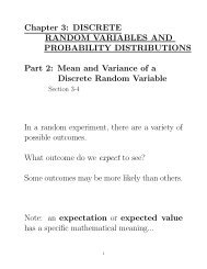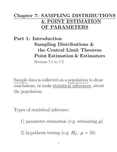
Chapter 7: SAMPLING DISTRIBUTIONS & POINT ESTIMATION OF ...

Chapter 7: SAMPLING DISTRIBUTIONS
& POINT ESTIMATION
OF PARAMETERS
Part 1: Introduction
Sampling Distributions &
the Central Limit Theorem
Point Estimation & Estimators
Sections 7-1 to 7-2
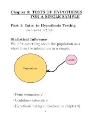
Sample data is collected on a population to draw
conclusions, or make statistical inferences, about
the population.
Types of statistical inference:
1) parameter estimation (e.g. estimating µ)
2) hypothesis testing (e.g. H 0 : µ = 50)
1

Example of parameter estimation
(or point estimation):
We’re interested in the value of µ.
The observed ¯x is a point estimate for µ.
µ is the parameter being estimated.
NOTATION: ˆµ = ¯X¯X is the estimator.
{We often show an estimator as a ‘hat’
over its respective parameter.}
The estimate is a single value,
or a point estimate.
¯X is the statistic of interest from the data.
2

Sample-to-sample variability
The value we get for ¯X (the sample mean) depends
on the sample chosen.
¯X is a random variable!
The distribution of ¯X is called the
sampling distribution of ¯X.
We expect ¯X to be close to µ (we ARE using
it to estimate µ) but there is variability in
¯X before it is observed because we use random
sampling to choose our sample of size n.
3

The sampling distribution of ¯X tells us what kind
of values are likely to occur for ¯X.
The sampling distribution of ¯X puts a probability
distribution on the possible values for ¯X.
In a simple random sample of n observations
from a population,
E( ¯X) = µ
⇒ ¯X is an unbiased estimator of µ.
This gives us a measure of center for the sampling
distribution for ¯X, but what about the
variability of the ¯X random variable
4

Sampling distribution of ¯X
Case 1 Original population is normally distributed.
f(x)
x
The ¯x I observe depends on the sample (the
particular n observations) I chose from this
normal distribution.
Let’s look at the distribution of ¯x values if I
choose a sample of size n and compute ¯x for
that sample, and I repeat this process 1000
times...
5

f(x)
x
1) Choose a sample of size n from a normal
distribution
2) Compute ¯x
3) Plot the ¯x on our frequency histogram
4) Do steps 1-3 1000 times
See applet at:
http://onlinestatbook.com/stat sim/sampling dist/index.html
6

SKETCH THE PLOTS:
Distribution of ¯X for n=2 when original population
is normal.
Distribution of ¯X for n=25 when original
population is normal.
7

Turns out, in this case, the the random variable
¯X is normally distributed.
This normal distribution is centered at µ (the
mean of the original population we were sampling
from).
The variability of ¯X depends on the sample
size n, and the variability in the original population.
SPECIFICALLY:
When X ∼ N(µ, σ 2 ),
¯X ∼ N(µ, σ2
n )
NOTE: the distribution for ¯X is less variable
than the distribution for X.
8

¯X ∼ N(µ, σ2
n )
NOTE: ¯X from n = 25 is less variable than
¯X from n = 2.
More data (larger n) gives us a better estimate
of µ from ¯X.
The distribution of our estimator ¯X is squished
closer, or is tighter, around the thing we’re
trying to estimate. Which is beneficial when
estimating something.
9

Sampling distribution of ¯X
Case 2 Original population is NOT normally
distributed.
f(x)
f(x)
x
x
f(x)
x
Or anything else...
10

What does the distribution of ¯X look like
1) Choose a sample of size n
from the distribution
2) Compute ¯x
3) Plot the ¯x on our frequency histogram
4) Do steps 1-3 1000 times
———————————————————–
Right-skewed with n = 10.
11

Really non-normal (mass out at the ends)
with n = 2.
Really non-normal (mass out at the ends)
with n = 25.
12

Turns out the random variable ¯X is normally
distributed no matter what your original distribution
was IF n is large enough...
What’s large enough
Rule of thumb is n ≥ 30
So, what have we learned...
if X is normally distributed, then
¯X ∼ N(µ, σ 2 /n) for any n.
if X is NOT normally distributed, then
¯X ∼ N(µ, σ 2 /n) for n ≥ 30.
if X is not severely non-normal, then
¯X ∼ N(µ, σ 2 /n) is close to true for n < 30.
13

Sampling Distributions and
the Central Limit Theorem
Section 7-2
Sample data is collected on a population to draw
conclusions, or make statistical inferences, about
the population.
NOTATION:
− A large letter like ¯X represents the random
variable ¯X, and ¯X can take on many values.
− A small letter like ¯x represents an actual observed
¯x from a sample, and it is a fixed
quanitity once observed.
14

• Random Sample
The random variables X 1 , X 2 , . . . , X n are a
random sample of size n if...
a) the X i ’s are independent random variables,
and
b) every X i has the same sample probability
distribution (i.e. they are drawn from the
same population).
NOTE: the observed data x 1 , x 2 , . . . , x n is
also referred to as a random sample.
15

• Statistic
– A statistic is any function of the observations
in a random sample.
∗ Example:
The mean ¯X is a function of the observations
(specifically, a linear combination
of the observations).
¯X =
∑ ni=1
X i
n
= 1 n X 1+ 1 n X 2+· · ·+ 1 n X n
– A statistic is a random variable,
and it has a probability distribution
– The distribution of a statistic is called the
sampling distribution of the statistic
because is depends on the sample chosen.
16

– The sampling distribution of the mean
is very important.
What is the expected value of the sample
mean ¯X in a random sample
E( ¯X) = E( 1 n X 1 + 1 n X 2 + · · · + 1 n X n)
= 1 ∑
E(Xi )
n
= 1 ∑ nµ µ =
n n = µ = µ ¯X
Notation: E( ¯X) = µ ¯X = µ
where µ is the population mean.
(µ is also the expected value
of a single X i )
17

What is the variance of the sample mean
¯X in a random sample
V ( ¯X) = V ( 1 n X 1 + 1 n X 2 + · · · + 1 n X n)
=
=
=
( ) 1 2 ∑
V (Xi )
n
( ) 1 2 ∑
σ
2
n
( 1
n) 2
nσ 2 = σ2
n
Notation: V ( ¯X) = σ 2¯X = σ2
n
where σ 2 is the population variance.
(σ 2 is also the variance of a single X i )
18

As we have described earlier, for n ≥ 30
¯X ∼ N(µ, σ2
n )
(and this is also true for n < 30 if each X i comes
from a normal population).
Using this fact, and what we know about standardizing
variables, leads to...
• The Central Limit Theorem
If X 1 , X 2 , . . . , X n is a random sample of size
n taken from a population with mean µ and
variance σ 2 , the limiting form of the distribution
of
Z = ¯X − µ
σ/ √ n
as n → ∞ is the standard normal distribution,
or N(0, 1).
19

The approximation of
¯X − µ
σ/ √ n
∼ N(0, 1)
depends on the size of n.
Satisfactory approximation for n ≥ 30 for
any population.
Satisfactory approximation for n < 30 for
near normal populations.
————————————————————
The next graphic shows 3 different original populations
(one nearly normal, two that are not),
and the sampling distribution for ¯X based on a
sample of size n = 5 and size n = 30.
20

The three original distributions are on the far
left (one that is nearly symmetric and bell-shaped,
one that is right skewed, and one that is highly
right skewed).
As shown in: Navidi, W. ‘Statistics for Engineers and Scientists’, McGraw Hill, 2006
21

Things to notice from the previous graphic:
• The variability of ¯X decreases as n increases
Recall: V ( ¯X) = σ2
n .
• If the original population has a shape that’s
closer to normal, smaller n is sufficient for ¯X
to be normal.
• The normal approximation gets better with
larger n when you’re starting with a nonnormal
population.
• Even when X has a very non-normal distribution,
¯X still has a normal distribution with
a large enough n.
22

• Example: Flaws in a copper wire.
Let X denote the number of flaws in a 1 inch
length of copper wire. The probability mass
function of X is presented in the following table:
x P (X = x)
0 0.48
1 0.39
2 0.12
3 0.01
Suppose n = 100 wires are sampled from this
population. What is the probability that the
average number of flaws per wire in the sample
is less than 0.5
23

ANS:
P ( ¯X < 0.5) =
24

Differences in sample means ¯X 1 and ¯X 2
What if we’re interested in estimating the difference
in means between two populations
Value of interest: µ 1 − µ 2
Estimator: ¯X1 − ¯X 2
0.00 0.05 0.10 0.15 0.20
Pop'n 1 Pop'n 2
−5 0 5 10 15 20 25 30
Y
The above picture shows two populations with
different means,
µ 1 − µ 2 ≠ 0.
25

0.00 0.05 0.10 0.15 0.20
Pop'n 1 Pop'n 2
−5 0 5 10 15 20 25 30
Y
If the populations had the same mean, then the
two distributions would be on top of each other
(no distinction), and µ 1 − µ 2 = 0.
We want to know the behavior of our estimator
¯X 1 − ¯X 2 .
So far, we’ve only discussed the behavior of ¯X.
26

The sampling distribution of ¯X1 − ¯X 2 :
We will assume the sample from each group was
taken independent of each other (two independent
samples).
E( ¯X 1 − ¯X 2 ) = E( ¯X 1 ) − E( ¯X 2 )
= µ 1 − µ 2
where µ 1 is the population mean of pop’n 1
where µ 2 is the population mean of pop’n 2
V ( ¯X 1 − ¯X 2 ) = V ( ¯X 1 ) + V ( ¯X 2 )
{since independent}
= σ2 1
n 1
+ σ2 2
n 2
where σ 2 1
where σ 2 2
is the population variance of pop’n 1
is the population variance of pop’n 2
27

⇒
¯X 1 − ¯X 2 is a random variable
with E( ¯X 1 − ¯X 2 ) = µ 1 − µ 2
and V ( ¯X 1 − ¯X 2 ) = σ2 1
n 1
+ σ2 2
n 2
So, we have the expected value and the variance
of this random variable of interest. But we’d like
to know the full distribution of the r.v.
28

IF both original populations were normal, then
¯X 1 and ¯X 2 are linear combinations of normal
random variables, and ¯X 1 − ¯X 2 is also a linear
combination of normals... so
¯X 1 − ¯X 2 ∼ N(µ 1 − µ 2 , σ2 1
n 1
+ σ2 2
n 2
)
Again, we have a random variable of interest
¯X 1 − ¯X 2 that has a normal distribution with
known ‘predictable’ behavior.
————————————————————
What if both original populations were NOT normal
If n 1 and n 2 are both greater than 30, then we
can apply the central limit theorem to show that
¯X 1 − ¯X 2 is again, normally distributed.
29

• Approximate Sampling Distribution
for ¯X 1 − ¯X 2
If we have two independent populations with
means µ 1 and µ 2 and variances σ 2 1 and σ2 2 ,
and if ¯X1 and ¯X 2 are sample means of two
independent random samples of size n 1 and
n 2 from the two populations, then the sampling
distribution of
Z = ( ¯X 1 − ¯X 2 ) − (µ 1 − µ 2 )
√
σ 2 1
n 1
+ σ2 2
n 2
is approximately standard normal (if the conditions
of the central limit theorem apply).
If the original populations were normal to begin
with, then Z is exactly a standard normal.
30

• Example: Difference in means
A random sample of n 1 =20 observations are
taken from a normal population with mean
30. A random sample of n 2 =25 observations
are taken from a different normal population
with mean 27. Both populations have
σ 2 = 8.
What is the probability that ¯X1 − ¯X 2 exceeds
5
31

• Example: Picture tube brightness (problem
7-14 p.231)
A consumer electronics company is comparing
the brightness of two different types of
picture tubes. Type A is the present model,
and is thought to have a population mean
brightness of 100 and a known standard deviation
of 16. Type B has an unknown mean
brightness and standard deviation equal to
type A.
If µ B exceeds µ A , the manufacturer would
like to adopt type B for use.
A random sample of 25 is taken from each
type...
32

The observed difference in sample means is
¯x B − ¯x A = 6.75
(so, the sample mean brightness for type B
was higher than the sample mean for type A,
but is it high enough).
What decision should they make
33