Lab 4 Handout - Marrella

1
AOS 452 ­ Lab 9 Handout
GARP: GEMPAK Analysis and Rendering Program
October 22, 2009
Tip of the Day: Printing complex GEMPAK PostScript files can take a while. Use the lpq program to check on the
status of your print job. The –P flag tells the program which printer to check, so, for example, type lpq –P gpend to
check the printer in the Synoptic Lab, or type lpq –P synoptic to check the printer in Room 1443 (the old Synoptic
Lab).
INTRODUCTION
GEMPAK will be the main tool you use for data analysis in your group and individual case studies.
Today, however, we will explore a more user­friendly program that combines many of the GEMPAK
programs into one package–GARP. GARP can be thought of as a “point­and­click” version of
GEMPAK that presents a graphical user interface (GUI) instead of a list of parameters in individual
programs.
You may be asking yourself, “Why are we using the more complicated GEMPAK programs when
GARP is available” In short, GARP is much more restrictive in its manipulation and display of data
than the GEMPAK programs. It is also a little slow and buggy. Finally, a new program, called IDV,
is currently a better version of both GARP and Vis5D (to be explored in future labs [maybe]), so
GARP is a bit of a lame duck. I will warn you right now: Do not use GARP for any graphics you
will present in your case studies! GARP will be most useful in taking a first glance at data sets,
getting a quick idea of the current weather, creating overlays with satellite or radar data for map
discussions, and nowcasting/storm chasing base support. Using GARP for radar and satellite data is
okay, but be thoughtful while making your images
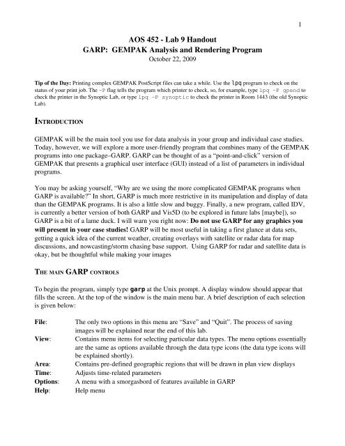
THE MAIN GARP CONTROLS
To begin the program, simply type garp at the Unix prompt. A display window should appear that
fills the screen. At the top of the window is the main menu bar. A brief description of each selection
is given below:
File:
View:
Area:
Time:
Options:
Help:
The only two options in this menu are “Save” and “Quit”. The process of saving
images will be explained near the end of this lab.
Contains menu items for selecting particular data types. The menu options essentially
are the same as options available through the data type icons (the data type icons will
be explained shortly).
Contains pre­defined geographic regions that will be drawn in plan view displays
Adjusts time­related parameters
A menu with a smorgasbord of features available in GARP
Help menu

2
Below the main menu bar, there are 10 data type icons. These icons are described below:
ICON 1
ICON 2
ICON 3
ICON 4
ICON 5
ICON 6
ICON 7
ICON 8
ICON 9
ICON 10
1 2 3 4 5 6 7 8 9 10
View satellite and radar imagery
View surface data plotted on a standard surface chart (similar to sfmap)
View wind profiler data (may not be currently available)
View upper air observational data plotted on a standard plan view upper­air chart or a
thermodynamic diagram (similar to snmap and snprof)
View horizontal plots of gridded (model) data sets (gdcntr, gdwind, or gdplot)
View vertical cross­sections using gridded (model) data (similar to gdcross)
View time­height sections
View vertical profile (sounding) plots from gridded (model) data (similar to gdprof)
Clear the graphics window (without clearing the map background)
Resets the graphics screen, so it appears as though you first began running GARP
In this lab, you will go through a few small exercises to familiarize yourself with a few of GARP's
capabilities. You can easily learn many of the other capabilities in GARP with a little experimenting.
MODEL PLAN PLOTS
To start things out, we are going to select a graphics area for a future plot. Drag the arrow to the
AREA menu on the main menu bar. Click on AREA and select CONUS. A map of the continental
United States should appear in the display window.
Now we are ready to choose a variable to plot. Click on the icon for horizontal plots using gridded
data (ICON 5) with the left mouse button. A window with the title “Model Plan View” will appear.
The next step is to select a model. Click and hold down the left mouse button on the upper­left box
where a model name (probably GFS thinned) is shown. A pull­down menu will appear with different
models listed. Select the Eta 211 model. (GARP hasn't been updated to reflect the name change yet.)
After possibly many seconds, you should see a list of date/time stamps in the column with the header
“Available Times” (or Date/Time). The date/time stamps are given in the following format:
yyyymmdd/ttttFTTT
yyyy = the four­digit year identifier
mm = the two­digit month identifier
dd = the two­digit day identifier
tttt = the hour of the model run (1200 = 1200 UTC, 0000 = 0000 UTC, etc.)
F = stands for forecast time
TTT = forecast hour (024 = 24­hour forecast time)

Note that the yyyymmdd/tttt tells the user from which model run the data are derived, or, in other
words, what day and time the model was initialized. The FTTT tells the user the forecast hour from
this model run. For example, 20091022/1200F012 would be the 12­hour forecast from the 1200 UTC
22 October 2009 model run, valid at 0000 UTC 23 October 2009. As such, not all the times listed
correspond to the same model run. Generally, you will want to use the most recent data available
(found at the bottom of the list).
Let’s try plotting geopotential height and absolute vorticity at 500 hPa using the 24­hour forecast
from the 1200 UTC 22 October 2009 Eta/NAM model run. Be sure to select the appropriate time,
pressure coordinate, level, correct functions, etc. You can always adjust the contour interval and
contour properties of the variables being plotted by selecting more on the lower right of the Model
Plan View box. Once you get the heights to plot overlay the absolute vorticity. See if you can get the
absolute vorticity to appear with color filling instead of contours.
NOTE: In GARP, it is easy to clear a variable that you plotted without clearing the entire screen.
Simply go to the bottom of the graphics window and single click the left mouse button on the title of
the variable you want taken off the screen. The title text will turn gray. You can bring the variable
back up onto the screen with a single click of the left mouse button on the grayed­out title.
FURTHER NOTE: In addition to selecting the already defined variables and functions, one can manually
enter a gfunc or gvect in the bottom part of the Model Plan View window.
Click ICON 9 to clear the graphics screen. Your plot should be cleared with only the background
map remaining.
3
LOOPING WITH GARP
In GARP, we can easily loop through a series of images, even with multiple overlays. We will now
make a loop of the visible satellite imagery with surface observations overlain. Use the Northeast
United States as the map background.
Click on the satellite and radar icon (ICON 1).
Select GOES­8 (this is actually GOES­12 data), 4 km, and VIS.
Click and hold the left mouse button on 20091022/1315 and drag down to the most recent time.
There should be about 7 forecast times highlighted.
Click the “Display and Close” button. You should see a series of satellite images plotted on the
screen.
Since we want to display surface observations taken around the same time the satellite pictures
were, we should use the “Time Matching” feature of GARP. In the Time menu, select Time
Matching, and then select Closest Time Match.
To overlay the surface obs, select ICON 2. Click Multi­color. Notice that the proper times are
already selected to match the satellite.

Click on the “Display and Close” button. The surface obs should overlay the satellite imagery.
Two methods can be used to loop through a series of images. You control the loop by clicking on
the buttons located to the right of the Speed and Fade slide bars in the top portion of the main
display window. The buttons look like the following:
4
Stepping through the frames one at a time
Clicking on the “” icon will bring up the next frame forward in time.
Looping through the frames
Clicking the “” will
loop the frames forward in time. Clicking the “” button will loop from the beginning frame
to the end frame, then loop back to the beginning frame. To stop the loop, click on the button
with the square.
DEFINING THE GRAPHICS AREA IN GARP
To begin this lab, you defined a graphics area covering the United States. Experiment with the other
graphics areas which are available from the area menu. Also, as in GEMPAK, you can zoom into an
area (and redefine the graphics area) by using the mouse. This is similar to the cursor command
covered in previous labs. Just create the box as if someone had already typed in the cursor command
for you, and GARP will automatically change the graphics area for you.
SAVING PLOTS IN GARP
If you are in a time crunch (and who isn't) and you want to create simple plots in GARP for your
map discussion, you will want to save the output. Once your plot (or loop) is complete, just click on
file and select save. Click on apply after creating the filename, and the file will be saved in your own
directory.
EXITING GARP
To exit GARP, click on quit from the file menu. It is not necessary to type gpend when exiting
GARP.

CREATING AN ANIMATION FROM A GARP LOOP
It is not too hard to convert a GARP loop into an FLI animation. Here's how:
0) As an example, create a loop of satellite imagery in GARP.
1) Click save from the file menu, just as if you were saving a plot. This time, though, click the
All Frames button.
2) Give your loop a filename, but without the .gif extension. For this example, just type sat.
3) Exit GARP
4) Type ls sat* and notice that GARP automatically numbered your images and supplied
the .gif extension.
5) Type file sat01.gif (for this example) and notice the image size.
6) Type ls -1 sat*.gif > sat_list This command lists in one column all files matching
sat*.gif, and places the output in a file called sat_list. (The ­1 is a number one).
7) Type cat sat_list to make sure the appropriate files are in your image list. If not, you'll
have to gedit the sat_list file.
8) For the final step, you'll type something like:
ppm2fli ­N ­g 1098x748 –fgiftopnm sat_list sat.fli
where 1098x748 should be replaced with the appropriate image size. This runs the FLI
conversion program, with ­N specifying that xanim will be able to play the loop backwards, ­g
###x### specifying the animation size, ­fgiftopnm specifying that the original images are
GIFs, sat_list specifying the list of images to convert to an animation, and sat.fli
specifying the name of the resulting animation.
Now you can type xanim sat.fli & to view your animation.
5