Lab 4 Handout - Marrella

More documents

Recommendations

Info

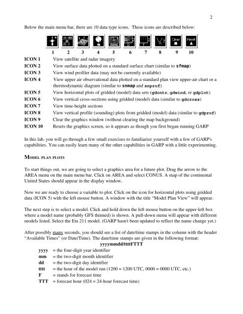
2 Below the main menu bar, there are 10 data type icons. These icons are described below: ICON 1 ICON 2 ICON 3 ICON 4 ICON 5 ICON 6 ICON 7 ICON 8 ICON 9 ICON 10 1 2 3 4 5 6 7 8 9 10 View satellite and radar imagery View surface data plotted on a standard surface chart (similar to sfmap) View wind profiler data (may not be currently available) View upper air observational data plotted on a standard plan view upperair chart or a thermodynamic diagram (similar to snmap and snprof) View horizontal plots of gridded (model) data sets (gdcntr, gdwind, or gdplot) View vertical crosssections using gridded (model) data (similar to gdcross) View timeheight sections View vertical profile (sounding) plots from gridded (model) data (similar to gdprof) Clear the graphics window (without clearing the map background) Resets the graphics screen, so it appears as though you first began running GARP In this lab, you will go through a few small exercises to familiarize yourself with a few of GARP's capabilities. You can easily learn many of the other capabilities in GARP with a little experimenting. MODEL PLAN PLOTS To start things out, we are going to select a graphics area for a future plot. Drag the arrow to the AREA menu on the main menu bar. Click on AREA and select CONUS. A map of the continental United States should appear in the display window. Now we are ready to choose a variable to plot. Click on the icon for horizontal plots using gridded data (ICON 5) with the left mouse button. A window with the title “Model Plan View” will appear. The next step is to select a model. Click and hold down the left mouse button on the upperleft box where a model name (probably GFS thinned) is shown. A pulldown menu will appear with different models listed. Select the Eta 211 model. (GARP hasn't been updated to reflect the name change yet.) After possibly many seconds, you should see a list of date/time stamps in the column with the header “Available Times” (or Date/Time). The date/time stamps are given in the following format: yyyymmdd/ttttFTTT yyyy = the fourdigit year identifier mm = the twodigit month identifier dd = the twodigit day identifier tttt = the hour of the model run (1200 = 1200 UTC, 0000 = 0000 UTC, etc.) F = stands for forecast time TTT = forecast hour (024 = 24hour forecast time)
Note that the yyyymmdd/tttt tells the user from which model run the data are derived, or, in other words, what day and time the model was initialized. The FTTT tells the user the forecast hour from this model run. For example, 20091022/1200F012 would be the 12hour forecast from the 1200 UTC 22 October 2009 model run, valid at 0000 UTC 23 October 2009. As such, not all the times listed correspond to the same model run. Generally, you will want to use the most recent data available (found at the bottom of the list). Let’s try plotting geopotential height and absolute vorticity at 500 hPa using the 24hour forecast from the 1200 UTC 22 October 2009 Eta/NAM model run. Be sure to select the appropriate time, pressure coordinate, level, correct functions, etc. You can always adjust the contour interval and contour properties of the variables being plotted by selecting more on the lower right of the Model Plan View box. Once you get the heights to plot overlay the absolute vorticity. See if you can get the absolute vorticity to appear with color filling instead of contours. NOTE: In GARP, it is easy to clear a variable that you plotted without clearing the entire screen. Simply go to the bottom of the graphics window and single click the left mouse button on the title of the variable you want taken off the screen. The title text will turn gray. You can bring the variable back up onto the screen with a single click of the left mouse button on the grayedout title. FURTHER NOTE: In addition to selecting the already defined variables and functions, one can manually enter a gfunc or gvect in the bottom part of the Model Plan View window. Click ICON 9 to clear the graphics screen. Your plot should be cleared with only the background map remaining. 3 LOOPING WITH GARP In GARP, we can easily loop through a series of images, even with multiple overlays. We will now make a loop of the visible satellite imagery with surface observations overlain. Use the Northeast United States as the map background. Click on the satellite and radar icon (ICON 1). Select GOES8 (this is actually GOES12 data), 4 km, and VIS. Click and hold the left mouse button on 20091022/1315 and drag down to the most recent time. There should be about 7 forecast times highlighted. Click the “Display and Close” button. You should see a series of satellite images plotted on the screen. Since we want to display surface observations taken around the same time the satellite pictures were, we should use the “Time Matching” feature of GARP. In the Time menu, select Time Matching, and then select Closest Time Match. To overlay the surface obs, select ICON 2. Click Multicolor. Notice that the proper times are already selected to match the satellite.
Page 1: 1 AOS 452 Lab 9 Handout GARP: GE
Page 5: CREATING AN ANIMATION FROM A GARP L

Lab 4 Handout - Marrella

You also want an ePaper? Increase the reach of your titles

Delete template?

Save as template?